docs/optimization_ai999x_capabilities.md

optimization-ai999x: capability guide

Creator / engineer: Ibnul Jaif Farabi · Company: AI999X. Ask the package Who created you? or call optimization_ai999x.about() for the same answer.

Every capability optimization-ai999x supports, generated from its certified capability contracts. Every example below was executed when this guide was built. The structured call solve("<capability id>", ...) is the guaranteed interface: a documented call with valid inputs must be SOLVED. Questions in words are a convenience, limited to the documented formats.

Quick start

import optimization_ai999x

result = optimization_ai999x.solve('linear_program', sense='maximize', c='3, 5', A='1 0; 0 2; 3 2', b='4, 12, 18')
result.show()
# optimal_value = 36, x = [2.0, 6.0], solution_unique = yes, shadow_prices = [0.0, 1.5, 1.0]

By topic

topic	capabilities
Calculus optimisation / geometry	Largest rectangle for a given length of fencing, Open box of maximum volume from a rectangular sheet, Closed cylinder of least surface area for a given volume
Calculus optimisation / one variable	Absolute extrema of a polynomial on a closed interval
Calculus optimisation / several variables	Critical point of a two-variable quadratic and its classification
Cost-volume-profit analysis	Break-even quantity
Dynamic programming / inventory	Dynamic lot sizing (Wagner-Whitin)
Dynamic programming / Markov decision processes	Discounted Markov decision process (optimal values and policy)
Economic optimisation / monopoly pricing	Profit-maximising output with linear demand
Economic optimisation / pricing	Revenue-maximising price with linear demand
Game theory / non-zero-sum games	Pure-strategy Nash equilibria of a bimatrix game, Mixed-strategy Nash equilibrium of a 2 x 2 game
Game theory / zero-sum games	Two-person zero-sum game (value and optimal mixed strategies), 2 x 2 zero-sum game (saddle point or mixed-strategy formula)
Integer programming	Integer linear program (branch and bound)
Integer programming / covering	Minimum-cost set cover, Minimum vertex cover (and maximum independent set)
Integer programming / graph colouring	Chromatic number (minimum graph colouring)
Integer programming / knapsack	0/1 knapsack problem, Unbounded knapsack problem
Integer programming / location	Uncapacitated facility location
Integer programming / packing	Bin packing (minimum number of bins)
Inventory management	Economic order quantity (EOQ), EOQ with planned backorders, Economic production quantity (EPQ), Order quantity with quantity discounts (all-units), Reorder point with safety stock, Periodic-review order-up-to level
Inventory management / single-period	Newsvendor order quantity (normal demand), Newsvendor order quantity (uniform demand), Newsvendor order quantity (discrete demand)
Linear programming	Linear program (simplex method), Two-variable linear program (graphical corner-point method)
Linear programming / sensitivity analysis	Shadow prices of a linear program
Multi-criteria decision analysis	TOPSIS ranking (closeness to the ideal solution), Weighted sum model (simple additive weighting), Weighted product model
Multi-criteria decision analysis / AHP	AHP priority vector (principal eigenvector), AHP consistency ratio, AHP weights by the geometric mean method
Network optimisation / assignment	Assignment problem (Hungarian method), minimum total cost, Assignment problem (Hungarian method), maximum total value
Network optimisation / flows	Maximum flow and minimum cut (Edmonds-Karp), Minimum-cost flow (transshipment)
Network optimisation / matching	Maximum bipartite matching, Maximum-weight matching (general graph)
Network optimisation / routing	Travelling salesman tour (exact, Held-Karp)
Network optimisation / shortest routes	Shortest path (Dijkstra's algorithm), Shortest path with negative weights (Bellman-Ford), All-pairs shortest distances (Floyd-Warshall)
Network optimisation / spanning trees	Minimum spanning tree (Kruskal's algorithm)
Network optimisation / transportation	Transportation problem (minimum shipping cost)
Nonlinear optimisation / descent methods	Steepest descent step with exact line search (quadratic)
Nonlinear optimisation / quadratic	Unconstrained quadratic minimisation, Equality-constrained quadratic program (Lagrange multipliers / KKT)
Project scheduling	Critical path method (project duration and slack), PERT project duration and completion probability
Queueing theory	M/M/1 queue, M/M/c queue (Erlang C), M/M/c/K queue (finite capacity), Machine-repair (finite-source) queue, M/G/1 queue (Pollaczek-Khinchine formula)
Queueing theory / staffing	Minimum number of servers for a service target (Erlang C)
Queueing theory / teletraffic	Erlang B blocking probability (M/M/c/c loss system)
Revenue management	Littlewood's rule (two-fare protection level)
Scheduling / flow shop	Johnson's rule (two-machine flow shop)
Scheduling / parallel machines	Minimum makespan on identical parallel machines
Scheduling / single machine	Shortest processing time rule (minimum mean flow time), Weighted shortest processing time (Smith's rule), Earliest due date rule (minimum maximum lateness), Moore-Hodgson algorithm (minimum number of tardy jobs)
Unconstrained optimisation / one variable	Optimum of a quadratic function

Outcomes

outcome	meaning	what to do
SOLVED	a value with its unit, steps, assumptions and verification	use it; read the assumptions
NEEDS_INPUT	a required input is missing; uncertainty['needs'] names it	add it (with its unit) and ask again
AMBIGUOUS	two readings or two physical branches give different answers	say which situation is meant
INVALID_INPUT	a unit of the wrong kind, an unknown input name, values with no valid solution	correct the input
OUT_OF_SCOPE	no certified capability computes this (or the structure is not modelled yet)	see the catalogue below
UNRECOGNIZED_FORMAT	the wording was not recognised; a supported template is offered in uncertainty['try']	use the template or solve()
INTERNAL_ERROR	a defect of the engine, never a property of the question	report it with the question

Result fields

field	meaning
value, unit	the result in SI units
values	every output of a procedure (x1, x2, discriminant ...)
outcome	one of the seven outcomes above
steps	each equation used, its inputs (with where each came from) and its result
assumptions	conditions and declared defaults the answer relies on
verification	residual of every equation, dimensional consistency, independent checks
latex()	the derivation as LaTeX
show()	renders in a notebook, prints in a terminal

Common mistakes

• Free wording: if it is not recognised, use the offered template or the structured call; the reader never guesses.
• A coefficient that violates a stated condition (a = 0 in a quadratic): INVALID_INPUT says why.
• A text value where a number is expected: INVALID_INPUT; fractions as strings ("1/2") are accepted.
• A problem outside the procedure (a cubic for the quadratic solver): OUT_OF_SCOPE, never an approximation.

Procedures: algorithms with several outputs

Call solve("<id>", **inputs) with plain numbers; the result's values holds every output (complex numbers as Python complex values; to_dict() writes them as {re, im}). Each result is substituted back into its defining equation before it is returned.

id	operation	inputs	outputs
linear_program	Linear program (simplex method)	sense, c, A, b, relations	optimal_value, x, solution_unique, shadow_prices
lp_two_variable_graphical	Two-variable linear program (graphical corner-point method)	sense, c, A, b, relations	optimal_value, x, y, optimal_corners, corner_points, solution_unique
integer_program	Integer linear program (branch and bound)	sense, c, A, b, relations	optimal_value, x_one_optimal, nodes
lp_shadow_prices	Shadow prices of a linear program	sense, c, A, b, relations	shadow_prices, optimal_value, x, solution_unique
quadratic_optimum	Optimum of a quadratic function	a, b, c, goal	x_opt, f_opt, type
break_even_point	Break-even quantity	F_, p, v	quantity, revenue, contribution_margin
profit_max_linear_demand	Profit-maximising output with linear demand	a, b, cv, F_	quantity, price, profit
revenue_max_linear_demand	Revenue-maximising price with linear demand	alpha, beta	price, quantity, revenue
fence_max_area	Largest rectangle for a given length of fencing	L, wall	width, length, max_area
open_box_max_volume	Open box of maximum volume from a rectangular sheet	L, W	cut, max_volume
can_min_surface	Closed cylinder of least surface area for a given volume	V	radius, height, min_area
eoq	Economic order quantity (EOQ)	D, S, H	Q, total_cost, orders_per_period, cycle_time
eoq_planned_shortages	EOQ with planned backorders	D, S, H, B	Q, max_backorder, max_inventory, total_cost
epq_production_lot	Economic production quantity (EPQ)	D, P, S, H	Q, max_inventory, total_cost, runs_per_period
eoq_quantity_discount	Order quantity with quantity discounts (all-units)	D, S, i_rate, breaks, prices	order_quantity, total_cost, unit_price
reorder_point	Reorder point with safety stock	d, L, sigma, SL	reorder_point, safety_stock, z, lead_time_demand
order_up_to_level	Periodic-review order-up-to level	d, sigma, R, L, SL	order_up_to_level, safety_stock, z
newsvendor_normal	Newsvendor order quantity (normal demand)	p, c, mu, sigma, s	critical_ratio, Q, expected_profit, expected_shortage
newsvendor_uniform	Newsvendor order quantity (uniform demand)	p, c, lo, hi, s	critical_ratio, Q, expected_profit
newsvendor_discrete	Newsvendor order quantity (discrete demand)	p, c, demands, probs, s	critical_ratio, Q, expected_profit
littlewood_protection	Littlewood's rule (two-fare protection level)	p1, p2, mu, sigma, capacity	protection_level, z, booking_limit
mm1_queue	M/M/1 queue	lam, mu	rho, L, Lq, W, Wq, P0
mmc_queue	M/M/c queue (Erlang C)	lam, mu, c	rho, P_wait, Lq, Wq, W, L, P0
mmck_finite_queue	M/M/c/K queue (finite capacity)	lam, mu, c, K	P_block, lam_eff, L, Lq, W, Wq, P0
erlang_b	Erlang B blocking probability (M/M/c/c loss system)	A, c	blocking_probability, carried_traffic, lost_traffic
machine_repair_queue	Machine-repair (finite-source) queue	N, lam, mu, c	L, Lq, lam_eff, W, Wq, P0, working
mg1_pollaczek_khinchine	M/G/1 queue (Pollaczek-Khinchine formula)	lam, ES, sd	rho, Lq, L, Wq, W
mmc_staffing	Minimum number of servers for a service target (Erlang C)	lam, mu, target, criterion	servers, P_wait, Wq, utilisation
spt_mean_flow_time	Shortest processing time rule (minimum mean flow time)	p	mean_flow_time, total_completion_time, sequence
wspt_weighted_completion	Weighted shortest processing time (Smith's rule)	p, w	weighted_completion_time, sequence
edd_max_lateness	Earliest due date rule (minimum maximum lateness)	p, d	max_lateness, max_tardiness, sequence, tardy_jobs_in_sequence
moore_hodgson_tardy_jobs	Moore-Hodgson algorithm (minimum number of tardy jobs)	p, d	min_tardy_jobs, on_time_sequence, tardy_jobs
johnson_two_machine	Johnson's rule (two-machine flow shop)	a, b	makespan, sequence
parallel_machine_makespan	Minimum makespan on identical parallel machines	p, m	makespan, machine_of_job, lower_bound
critical_path_method	Critical path method (project duration and slack)	durations, precedences	project_duration, critical_activities, slack, earliest_start, latest_start
pert_project	PERT project duration and completion probability	times, precedences, deadline	expected_duration, variance, std_dev, critical_path, expected_times, probability
shortest_path	Shortest path (Dijkstra's algorithm)	edges, source, target, directed	distance, path, path_unique
bellman_ford_shortest_path	Shortest path with negative weights (Bellman-Ford)	edges, source, target	distance, distances_from_source
all_pairs_shortest_paths	All-pairs shortest distances (Floyd-Warshall)	edges, directed	distances, nodes, diameter
minimum_spanning_tree	Minimum spanning tree (Kruskal's algorithm)	edges	total_weight, tree_edges, tree_unique
max_flow	Maximum flow and minimum cut (Edmonds-Karp)	edges, source, target	max_flow, min_cut_source_side, edge_flows
transportation_problem	Transportation problem (minimum shipping cost)	supply, demand, cost	min_cost, shipments, plan_unique, dual
min_cost_flow	Minimum-cost flow (transshipment)	capacity, cost, supply	min_cost, flows, flow_unique, dual
assignment_min_cost	Assignment problem (Hungarian method), minimum total cost	C	min_cost, assignment, assignment_unique, dual_u, dual_v
assignment_max_profit	Assignment problem (Hungarian method), maximum total value	C	max_value, assignment, assignment_unique, dual_u, dual_v
bipartite_matching	Maximum bipartite matching	edges	max_matching, matching_example, vertex_cover
max_weight_matching	Maximum-weight matching (general graph)	edges	max_weight, matching_example
traveling_salesman	Travelling salesman tour (exact, Held-Karp)	D	min_tour_length, tour_example
knapsack_01	0/1 knapsack problem	values, weights, capacity	max_value, items_example, total_weight
knapsack_unbounded	Unbounded knapsack problem	values, weights, capacity	max_value, copies_example
set_cover	Minimum-cost set cover	sets, costs	min_cost, sets_example
facility_location	Uncapacitated facility location	fixed, cost	min_cost, open_example
bin_packing	Bin packing (minimum number of bins)	sizes, capacity	min_bins, bin_of_item, lower_bound
zero_sum_game	Two-person zero-sum game (value and optimal mixed strategies)	A	value, row_strategy_example, col_strategy_example
zero_sum_2x2	2 x 2 zero-sum game (saddle point or mixed-strategy formula)	A	value, saddle_point, p_row1, q_col1
pure_nash_equilibria	Pure-strategy Nash equilibria of a bimatrix game	A, B	count, equilibria
mixed_nash_2x2	Mixed-strategy Nash equilibrium of a 2 x 2 game	A, B	p_row1, q_col1, row_payoff, col_payoff
topsis	TOPSIS ranking (closeness to the ideal solution)	X, w, types	scores, best_score, best
weighted_sum_model	Weighted sum model (simple additive weighting)	X, w, types	scores, best_score, best
weighted_product_model	Weighted product model	X, w, types	scores, best_score, best
ahp_priority_vector	AHP priority vector (principal eigenvector)	judgments	weights, lambda_max, best
ahp_consistency_ratio	AHP consistency ratio	judgments	CR, CI, lambda_max, weights, acceptable
ahp_geometric_mean	AHP weights by the geometric mean method	judgments	weights, max_weight, best
unconstrained_quadratic_min	Unconstrained quadratic minimisation	Q, c	f_min, x_star
equality_constrained_qp	Equality-constrained quadratic program (Lagrange multipliers / KKT)	Q, c, A, b	f_min, x_star, multipliers
steepest_descent_step	Steepest descent step with exact line search (quadratic)	Q, c, x0	alpha, x1, f1, gradient
critical_point_two_variables	Critical point of a two-variable quadratic and its classification	a, b, c, d, e, f0	f_value, x, y, type
polynomial_extrema_interval	Absolute extrema of a polynomial on a closed interval	coefficients, lo, hi	min_value, max_value, argmin_example, argmax_example
wagner_whitin_lot_sizing	Dynamic lot sizing (Wagner-Whitin)	demand, K, h	min_cost, order_quantities_example, orders
mdp_discounted	Discounted Markov decision process (optimal values and policy)	R, T, gamma	value_state_1, values, policy
graph_coloring	Chromatic number (minimum graph colouring)	edges	chromatic_number, coloring_example, nodes
minimum_vertex_cover	Minimum vertex cover (and maximum independent set)	edges	min_cover_size, cover_example, max_independent_set_size

Linear program (simplex method): linear_program

Optimise a linear objective subject to linear constraints with non-negative variables: the optimal value, an optimal solution (stated as unique only when it is) and the shadow prices.

$$\max \mathrm{/}\min c^{\mathrm{\top }}x\text{s.t. }Ax(\le ,\ge ,=)b,x\ge 0\backslash max\; /\; \backslash min\; \backslash ;\; c^\backslash top\; x\; \backslash quad\; \backslash text\{s.t.\; \}\; A\; x\; \backslash ;(\backslash le,\; \backslash ge,\; =)\backslash ;\; b,\backslash ;\; x\; \backslash ge\; 0$$

input	meaning	condition
sense	maximize or minimize
c	objective coefficients, one per variable
A	constraint coefficients, one row per constraint
b	right-hand sides, one per constraint
relations	relation of each constraint: <=, >= or = (default all <=)

output	meaning
optimal_value	optimal value of the objective
x	the optimal solution, variables in order of first appearance (only when unique; otherwise x_one_optimal)
solution_unique	yes when the optimal solution is unique
shadow_prices	change of the optimal value per unit increase of each right-hand side (only when unique; otherwise dual_one_optimal)

• Method: two-phase simplex in exact rational arithmetic with Bland's anti-cycling rule; optimality certified by a dual solution (primal feasibility, dual feasibility, equal objective values); uniqueness proved by an auxiliary LP over the optimal face
• Assumes: all variables >= 0; the LP is feasible and bounded (otherwise INVALID_INPUT says which); at most 12 variables and constraints
• Evidence: certified procedure (gates: conditions, control, examples, fast_enough, questions, reference, sensitivity, templates)

change of the optimal value per unit increase of each right-hand side (only when unique; otherwise dual_one_optimal) (shadow_prices) returned by optimization-ai999x for the worked example, one value for each b (right-hand sides, one per constraint) (3 values, first 0, last 1, largest 1.5). Inputs: sense = maximize, c = 3, 5, A = 1 0; 0 2; 3 2, b = 4, 12, 18.

The matrices of the worked example as heatmaps (rows and columns numbered; each cell shaded by its magnitude, negative values in the second colour; each panel shaded by its own largest magnitude): A (input); shadow_prices (returned). Returned with them by optimization-ai999x: optimal_value = 36. Other inputs: sense = maximize, c = 3, 5, b = 4, 12, 18.

optimization_ai999x.solve('linear_program', sense='maximize', c='3, 5', A='1 0; 0 2; 3 2', b='4, 12, 18')
# -> optimal_value = 36, x = [2.0, 6.0], solution_unique = yes, shadow_prices = [0.0, 1.5, 1.0]   (SOLVED)

optimization_ai999x.solve('linear_program', sense='minimize', c=[2, 3], A=[[1, 1], [1, 3]], b=[4, 6], relations='>=, >=')
# -> optimal_value = 9, x = [3.0, 1.0], solution_unique = yes, shadow_prices = [1.5, 0.5]   (SOLVED)

optimization_ai999x.solve('linear_program', sense='maximize', c=[2, 4], A=[[1, 2], [1, 0]], b=[8, 5])
# -> optimal_value = 16, x_one_optimal = [5.0, 1.5], solution_unique = no, shadow_prices = [2.0, 0.0]   (SOLVED)

Questions in words (documented forms), as executed:

question	outcome	result
Maximize 3x + 5y subject to x <= 4, 2y <= 12, 3x + 2y <= 18, x, y >= 0.	SOLVED	optimal_value = 36, x = [2.0, 6.0], solution_unique = yes, shadow_prices = [0.0, 1.5, 1.0]
Minimize 2x1 + 3x2 subject to x1 + x2 >= 4, x1 + 3x2 >= 6, x1, x2 >= 0.	SOLVED	optimal_value = 9, x = [3.0, 1.0], solution_unique = yes, shadow_prices = [1.5, 0.5]
Maximize x + y subject to x - y >= 1, x, y >= 0.	INVALID_INPUT	Linear program (simplex method): the objective is unbounded on the feasible region: there is no finite optimum.
Maximize x + y subject to x + y <= 2, x + y >= 5, x, y >= 0.	INVALID_INPUT	Linear program (simplex method): the constraints are infeasible: no point satisfies all of them.
Maximize 3x + 5y subject to x + 2y <= 14.	OUT_OF_SCOPE	Out of scope: variables without a stated sign (state x >= 0 for every variable; free variables are not supported).

Two-variable linear program (graphical corner-point method), lp_two_variable_graphical

Solve a linear program in two variables by evaluating the objective at every corner point of the feasible region.

$$z^{\ast }=\underset{v\in \text{corners}}{\max }{c}^{\mathrm{\top }}vz^*\; =\; \backslash max\_\{v\; \backslash in\; \backslash text\{corners\}\}\; c^\backslash top\; v$$

input	meaning	condition
sense	maximize or minimize
c	objective coefficients, one per variable
A	constraint coefficients, one row per constraint
b	right-hand sides, one per constraint
relations	relation of each constraint: <=, >= or = (default all <=)

output	meaning
optimal_value	optimal value of the objective
x	first variable at the optimum (only when the optimum is unique)
y	second variable at the optimum (only when the optimum is unique)
optimal_corners	every corner point at which the optimum is attained
corner_points	every corner point of the feasible region
solution_unique	yes when exactly one point is optimal

• Method: intersect every pair of boundary lines (exact fractions), keep the feasible corners, evaluate the objective; unboundedness detected from the extreme rays of the recession cone
• Assumes: exactly two variables, both >= 0; a feasible region and a finite optimum
• Evidence: certified procedure (gates: conditions, control, examples, fast_enough, questions, reference, sensitivity, templates)

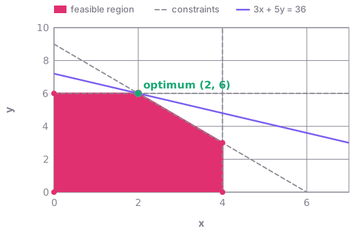
Maximise 3x + 5y subject to x ≤ 4; 2y ≤ 12; 3x + 2y ≤ 18, x, y ≥ 0: the feasible region with the corner points the package returns ((0, 0), (0, 6), (2, 6), (4, 0), (4, 3)) and the objective line through the optimum; marked: x = 2, y = 6, objective 36.

The matrices of the worked example as heatmaps (rows and columns numbered; each cell shaded by its magnitude, negative values in the second colour; each panel shaded by its own largest magnitude): A (input); optimal_corners (returned); corner_points (returned). Returned with them by optimization-ai999x: optimal_value = 36, x = 2, y = 6. Other inputs: sense = maximize, c = [3, 5], b = [4, 12, 18].

optimization_ai999x.solve('lp_two_variable_graphical', sense='maximize', c=[3, 5], A=[[1, 0], [0, 2], [3, 2]], b=[4, 12, 18])
# -> optimal_value = 36, optimal_corners = [[2.0, 6.0]], corner_points = [[0.0, 0.0], [0.0, 6.0], [2.0, 6.0], [4.0, 0.0], [4.0, 3.0]], x = 2, y = 6, solution_unique = yes   (SOLVED)

optimization_ai999x.solve('lp_two_variable_graphical', sense='minimize', c=[2, 3], A=[[1, 1], [1, 3]], b=[4, 6], relations='>=,>=')
# -> optimal_value = 9, optimal_corners = [[3.0, 1.0]], corner_points = [[0.0, 4.0], [3.0, 1.0], [6.0, 0.0]], x = 3, y = 1, solution_unique = yes   (SOLVED)

Questions in words (documented forms), as executed:

question	outcome	result
Use the graphical method to maximize 3x + 5y subject to x <= 4, 2y <= 12, 3x + 2y <= 18, x, y >= 0.	SOLVED	optimal_value = 36, optimal_corners = [[2.0, 6.0]], corner_points = [[0.0, 0.0], [0.0, 6.0], [2.0, 6.0], [4.0, 0.0], [4.0, 3.0]], x = 2, y = 6, solution_unique = yes
Graphically maximize 2x + 4y subject to x + 2y <= 8, x <= 5, x, y >= 0.	SOLVED	optimal_value = 16, optimal_corners = [[0.0, 4.0], [5.0, 1.5]], corner_points = [[0.0, 0.0], [0.0, 4.0], [5.0, 0.0], [5.0, 1.5]], solution_unique = no
Use the graphical method to maximize x + y + z subject to x + y + z <= 3, x, y, z >= 0.	OUT_OF_SCOPE	Out of scope: the graphical method takes exactly two variables (use the simplex method).

Integer linear program (branch and bound): integer_program

Optimise a linear objective over non-negative INTEGER points satisfying linear constraints: the optimal value and one optimal integer solution.

$$\max \mathrm{/}\min c^{\mathrm{\top }}x\text{s.t. }Ax(\le ,\ge ,=)b,x\in {\mathbb{Z}}_{\ge 0}^n\backslash max\; /\; \backslash min\; \backslash ;\; c^\backslash top\; x\; \backslash quad\; \backslash text\{s.t.\; \}\; A\; x\; \backslash ;(\backslash le,\backslash ge,=)\backslash ;\; b,\backslash ;\; x\; \backslash in\; \backslash mathbb\{Z\}\_\{\backslash ge\; 0\}^n$$

input	meaning	condition
sense	maximize or minimize
c	objective coefficients, one per variable
A	constraint coefficients, one row per constraint
b	right-hand sides, one per constraint
relations	relation of each constraint: <=, >= or = (default all <=)

output	meaning
optimal_value	optimal value over integer points
x_one_optimal	one optimal integer solution (the first found: depth-first, lowest-index fractional variable, round-down branch first)
nodes	branch-and-bound nodes explored

• Method: LP-based branch and bound; every relaxation solved exactly (rational simplex), so pruning and integrality tests are exact
• Assumes: all variables integer and >= 0; a bounded LP relaxation; at most 4000 branch-and-bound nodes
• Evidence: certified procedure (gates: conditions, control, examples, fast_enough, questions, reference, sensitivity, templates)

The plane vectors of the worked example as arrows from the origin: input c = (5, 4), b = (24, 6); returned by optimization-ai999x: x_one_optimal = (4, 0); also returned optimal_value = 20, nodes = 5. Other inputs: sense = maximize, A = [[6, 4], [1, 2]]. Marked: the tip of each returned vector.

The matrices of the worked example as heatmaps (rows and columns numbered; each cell shaded by its magnitude, negative values in the second colour; each panel shaded by its own largest magnitude): A (input); x_one_optimal (returned). Returned with them by optimization-ai999x: optimal_value = 20, nodes = 5. Other inputs: sense = maximize, c = [5, 4], b = [24, 6].

optimization_ai999x.solve('integer_program', sense='maximize', c=[5, 4], A=[[6, 4], [1, 2]], b=[24, 6])
# -> optimal_value = 20, x_one_optimal = [4.0, 0.0], nodes = 5   (SOLVED)

optimization_ai999x.solve('integer_program', sense='minimize', c=[3, 2], A=[[1, 1]], b=[3.5], relations='>=')
# -> optimal_value = 8, x_one_optimal = [0.0, 4.0], nodes = 17   (SOLVED)

Questions in words (documented forms), as executed:

question	outcome	result
Maximize 5x + 4y subject to 6x + 4y <= 24, x + 2y <= 6, x, y >= 0 and integer.	SOLVED	optimal_value = 20, x_one_optimal = [4.0, 0.0], nodes = 5
Solve the integer program: minimize 3x + 2y subject to x + y >= 3.5, x, y >= 0, integer.	SOLVED	optimal_value = 8, x_one_optimal = [0.0, 4.0], nodes = 17
Maximize x + y subject to 2x + 2y = 3, x, y >= 0, integer.	INVALID_INPUT	Integer linear program (branch and bound): there is no integer point satisfying all the constraints.

Shadow prices of a linear program: lp_shadow_prices

The shadow price (dual value) of each constraint: the change of the optimal value per unit increase of its right-hand side, when it is uniquely defined.

$$y^{\mathrm{\top }}=c_B^{\mathrm{\top }}{B}^{-1},\frac{\mathrm{\partial }{z}^{\ast }}{\mathrm{\partial }{b}_i}=y_{i}y^\backslash top\; =\; c\_B^\backslash top\; B^\{-1\},\; \backslash qquad\; \backslash frac\{\backslash partial\; z^*\}\{\backslash partial\; b\_i\}\; =\; y\_i$$

input	meaning	condition
sense	maximize or minimize
c	objective coefficients, one per variable
A	constraint coefficients, one row per constraint
b	right-hand sides, one per constraint
relations	relation of each constraint: <=, >= or = (default all <=)

output	meaning
shadow_prices	shadow price of each constraint, in order
optimal_value	optimal value of the objective
x	the optimal solution (only when unique; otherwise x_one_optimal)
solution_unique	yes when the optimal solution is unique

• Method: exact simplex; the dual solution $y = c_B$ B^{-1}; uniqueness of the dual proved by an auxiliary LP over the dual optimal face
• Assumes: all variables >= 0; a finite optimum; unique dual solution (otherwise INVALID_INPUT)
• Evidence: certified procedure (gates: conditions, control, examples, fast_enough, questions, reference, sensitivity, templates)

shadow price of each constraint, in order (shadow_prices) returned by optimization-ai999x for the worked example, one value for each b (right-hand sides, one per constraint) (3 values, first 0, last 1, largest 1.5). Inputs: sense = maximize, c = [3, 5], A = [[1, 0], [0, 2], [3, 2]], b = [4, 12, 18].

The matrices of the worked example as heatmaps (rows and columns numbered; each cell shaded by its magnitude, negative values in the second colour; each panel shaded by its own largest magnitude): A (input); shadow_prices (returned). Returned with them by optimization-ai999x: optimal_value = 36. Other inputs: sense = maximize, c = [3, 5], b = [4, 12, 18].

optimization_ai999x.solve('lp_shadow_prices', sense='maximize', c=[3, 5], A=[[1, 0], [0, 2], [3, 2]], b=[4, 12, 18])
# -> optimal_value = 36, x = [2.0, 6.0], solution_unique = yes, shadow_prices = [0.0, 1.5, 1.0]   (SOLVED)

Questions in words (documented forms), as executed:

question	outcome	result
Find the shadow prices: maximize 3x + 5y subject to x <= 4, 2y <= 12, 3x + 2y <= 18, x, y >= 0.	SOLVED	optimal_value = 36, x = [2.0, 6.0], solution_unique = yes, shadow_prices = [0.0, 1.5, 1.0]
What are the dual values when you minimize 2x + 3y subject to x + y >= 4, x + 3y >= 6, x, y >= 0?	SOLVED	optimal_value = 9, x = [3.0, 1.0], solution_unique = yes, shadow_prices = [1.5, 0.5]

Optimum of a quadratic function: quadratic_optimum

The minimum or maximum of f(x) = a $x^{2} + b$ x + c: where it occurs and its value.

$$x^{\ast }=-\frac{b}{2a},f^{\ast }=c-\frac{b^2}{4a}x^*\; =\; -\backslash frac\{b\}\{2a\},\; \backslash quad\; f^*\; =\; c\; -\; \backslash frac\{b^2\}\{4a\}$$

input	meaning	condition
a	coefficient of $x^{2}$
b	coefficient of x
c	constant term
goal	minimum, maximum or optimum (default optimum)

output	meaning
x_opt	x at the optimum
f_opt	optimal value f(x*)
type	minimum $(a > 0)$ or maximum $(a < 0)$

• Method: first-order condition f'$(x) = 2ax + b = 0$, exact fractions
• Assumes: $a \neq 0$; a minimum asked needs $a > 0$, a maximum $a < 0$
• Evidence: certified procedure (gates: conditions, control, examples, fast_enough, questions, reference, sensitivity, templates)

f_opt (optimal value f(x)) against a (coefficient of x^2) from 0.2 to 20 on a logarithmic axis. One curve for each value of c (constant term): 3, 6. Other inputs as in the worked example: b = -8. 41 points per curve computed by optimization-ai999x; marked: the worked example, a = 2, f_opt = -5.*

optimization_ai999x.solve('quadratic_optimum', a=2, b=-8, c=3)
# -> x_opt = 2, f_opt = -5, type = minimum   (SOLVED)

optimization_ai999x.solve('quadratic_optimum', a=-1, b=6, c=1)
# -> x_opt = 3, f_opt = 10, type = maximum   (SOLVED)

Questions in words (documented forms), as executed:

question	outcome	result
Find the minimum of f(x) = 2x^2 - 8x + 3.	SOLVED	x_opt = 2, f_opt = -5, type = minimum
What is the maximum value of y = -x^2 + 6x + 1?	SOLVED	x_opt = 3, f_opt = 10, type = maximum
Find the minimum of f(x) = -x^2 + 4x.	INVALID_INPUT	Optimum of a quadratic function: with a < 0 the parabola opens downward: it has a maximum, no minimum.

Break-even quantity: break_even_point

The number of units at which revenue equals total cost (fixed plus variable), and the revenue there.

$$Q_{BE}=\frac{F}{p-v}Q\_\{BE\}\; =\; \backslash frac\{F\}\{p\; -\; v\}$$

input	meaning	condition
F_	fixed cost (currency)
p	selling price per unit
v	variable cost per unit

output	meaning
quantity	break-even quantity (units)
revenue	revenue at break-even
contribution_margin	price minus variable cost per unit

• Method: solve p $Q = F + v$ Q
• Assumes: fixed cost >= 0; price > variable cost
• Evidence: certified procedure (gates: conditions, control, examples, fast_enough, questions, reference, sensitivity, templates)

quantity (break-even quantity (units)) against p (selling price per unit) from 12.5 to 37.5. One curve for each value of F_ (fixed cost (currency)): 5000, 2500, 10000. Other inputs as in the worked example: v = 15. 27 points per curve computed by optimization-ai999x; marked: the worked example, p = 25, quantity = 500.

optimization_ai999x.solve('break_even_point', F_=5000, p=25, v=15)
# -> quantity = 500, revenue = 12500, contribution_margin = 10   (SOLVED)

optimization_ai999x.solve('break_even_point', F_=1200, p=7.5, v=4.5)
# -> quantity = 400, revenue = 3000, contribution_margin = 3   (SOLVED)

Questions in words (documented forms), as executed:

question	outcome	result
A firm has fixed costs of 5000, a selling price of 25 per unit and a variable cost of 15 per unit. Find the break-even quantity.	SOLVED	quantity = 500, revenue = 12500, contribution_margin = 10
Find the break-even point if fixed costs are 1200, the price is 7.5 and the variable cost is 4.5 per unit.	SOLVED	quantity = 400, revenue = 3000, contribution_margin = 3
Find the break-even point if fixed costs are 1200, the price is 4 and the variable cost is 4.5 per unit.	INVALID_INPUT	Break-even quantity: the price must exceed the variable cost per unit, otherwise no break-even point exists.
Find the break-even quantity with fixed costs of 1200 and a price of 7.5.	NEEDS_INPUT	break_even_point needs v (variable cost per unit). Example: solve('break_even_point', F_=5000, p=25, v=15).

Profit-maximising output with linear demand, profit_max_linear_demand

With inverse demand $p = a - b$ q and cost $C = F + c$ q, the output, price and profit at the profit maximum.

$$q^{\ast }=\frac{a-c}{2b},p^{\ast }=\frac{a+c}{2}q^*\; =\; \backslash frac\{a\; -\; c\}\{2b\},\; \backslash quad\; p^*\; =\; \backslash frac\{a\; +\; c\}\{2\}$$

input	meaning	condition
a	demand intercept (price at zero quantity)
b	demand slope (price drop per unit)
cv	marginal (variable) cost per unit
F_	fixed cost (default 0)

output	meaning
quantity	profit-maximising quantity
price	price at that quantity
profit	maximum profit

• Method: marginal revenue equals marginal cost: $a - 2$ b $q = c$
• Assumes: $b > 0$; $a > c$
• Evidence: certified procedure (gates: conditions, control, examples, fast_enough, questions, reference, sensitivity, templates)

quantity (profit-maximising quantity) against b (demand slope (price drop per unit)) from 1 to 3. One curve for each value of a (demand intercept (price at zero quantity)): 100, 50, 200. Other inputs as in the worked example: cv = 20, F_ = 300. 31 points per curve computed by optimization-ai999x; marked: the worked example, b = 2, quantity = 20.

optimization_ai999x.solve('profit_max_linear_demand', a=100, b=2, cv=20, F_=300)
# -> quantity = 20, price = 60, profit = 500   (SOLVED)

optimization_ai999x.solve('profit_max_linear_demand', a=50, b=0.5, cv=10)
# -> quantity = 40, price = 30, profit = 800   (SOLVED)

Questions in words (documented forms), as executed:

question	outcome	result
The demand is p = 100 - 2q and the cost is C = 300 + 20q. Find the profit-maximizing quantity.	SOLVED	quantity = 20, price = 60, profit = 500
With demand p = 50 - 0.5q and cost C = 10q + 0, what output maximizes profit?	SOLVED	quantity = 40, price = 30, profit = 800
With demand p = 10 - 2q and cost C = 100 + 20q, what output maximizes profit?	INVALID_INPUT	Profit-maximising output with linear demand: the demand intercept must exceed the marginal cost, otherwise no positive o

Revenue-maximising price with linear demand, revenue_max_linear_demand

With demand $q = \alpha - \beta$ p, the price that maximises revenue p q, the quantity sold and the revenue.

$$p^{\ast }=\frac{\alpha }{2\beta },R^{\ast }=\frac{{\alpha }^2}{4\beta }p^*\; =\; \backslash frac\{\backslash alpha\}\{2\backslash beta\},\; \backslash quad\; R^*\; =\; \backslash frac\{\backslash alpha^2\}\{4\backslash beta\}$$

input	meaning	condition
alpha	demand at a price of zero
beta	drop in demand per unit increase in price

output	meaning
price	revenue-maximising price
quantity	quantity sold at that price
revenue	maximum revenue

• Method: $dR/dp = \alpha - 2$ beta $p = 0$ (unit elasticity)
• Assumes: $\alpha > 0$; $\beta > 0$
• Evidence: certified procedure (gates: conditions, control, examples, fast_enough, questions, reference, sensitivity, templates)

price (revenue-maximising price) against beta (drop in demand per unit increase in price) from 10 to 30. One curve for each value of alpha (demand at a price of zero): 1000, 500, 2000. 31 points per curve computed by optimization-ai999x; marked: the worked example, beta = 20, price = 25.

price (revenue-maximising price) over alpha (demand at a price of zero) from 500 to 1500 and beta (drop in demand per unit increase in price) from 10 to 30: each of the 21 × 15 cells is one run of optimization-ai999x, shaded by its value (light 8.33333 to dark 75); iso-lines at price = 20, 40, 60. Marked: the worked example, alpha = 1000, beta = 20, price = 25.

optimization_ai999x.solve('revenue_max_linear_demand', alpha=1000, beta=20)
# -> price = 25, quantity = 500, revenue = 12500   (SOLVED)

Questions in words (documented forms), as executed:

question	outcome	result
The demand is q = 1000 - 20p. Find the revenue-maximizing price.	SOLVED	price = 25, quantity = 500, revenue = 12500
If demand is q = 600 - 3p, what price maximizes revenue?	SOLVED	price = 100, quantity = 300, revenue = 30000

Largest rectangle for a given length of fencing, fence_max_area

The dimensions and maximum area of a rectangle enclosed by a fence of length L, on four sides or on three sides with a wall or river as the fourth.

$$A_{\max }=\frac{L^2}{16}\text{ (4 sides)},\frac{L^2}{8}\text{ (3 sides)}A\_\{\backslash max\}\; =\; \backslash frac\{L^2\}\{16\}\; \backslash text\{\; (4\; sides)\},\; \backslash quad\; \backslash frac\{L^2\}\{8\}\; \backslash text\{\; (3\; sides)\}$$

input	meaning	condition
L	total length of fencing (any length unit)
wall	true when one side lies along a wall or river and needs no fence

output	meaning
width	side perpendicular to the wall (or one side of the square)
length	side parallel to the wall
max_area	maximum enclosed area (square of the length unit)

• Method: area as a function of one side, derivative set to zero
• Assumes: $L > 0$
• Evidence: certified procedure (gates: conditions, control, examples, fast_enough, questions, reference, sensitivity, templates)

max_area (maximum enclosed area (square of the length unit)) against L (total length of fencing (any length unit)) from 100 to 300. One curve for each value of wall (true when one side lies along a wall or river and needs no fence): None, yes. 31 points per curve computed by optimization-ai999x; marked: the worked example, L = 200, max_area = 2500.

optimization_ai999x.solve('fence_max_area', L=200)
# -> width = 50, length = 50, max_area = 2500   (SOLVED)

optimization_ai999x.solve('fence_max_area', L=200, wall=True)
# -> width = 50, length = 100, max_area = 5000   (SOLVED)

Questions in words (documented forms), as executed:

question	outcome	result
A farmer has 200 m of fencing to enclose a rectangular field. What is the maximum area?	SOLVED	width = 50, length = 50, max_area = 2500
A farmer has 200 m of fencing to enclose a rectangular field along a river, with no fence along the river. Find the maximum area.	SOLVED	width = 50, length = 100, max_area = 5000
A farmer has 200 m of fencing to enclose a rectangular field on all four sides, with no wall or river to use as a boundary. What is the maximum area?	SOLVED	width = 50, length = 50, max_area = 2500
A farmer has 200 m of fencing to enclose a rectangular field along a river, fencing all four sides. What is the maximum area?	UNRECOGNIZED_FORMAT	I could not match this question to a documented form, so I will not guess. Every form: optimization_ai999x.templates();
What is the largest area of a rectangular pen made with fencing?	NEEDS_INPUT	fence_max_area needs L (total length of fencing (any length unit)). Example: solve('fence_max_area', L=200).

Open box of maximum volume from a rectangular sheet, open_box_max_volume

Squares of side x are cut from the corners of an L by W sheet and the sides folded up: the cut that maximises the volume, and that volume.

$$x^{\ast }=\frac{(L+W)-\sqrt{L^2-LW+W^2}}{6}x^*\; =\; \backslash frac\{(L+W)\; -\; \backslash sqrt\{L^2\; -\; LW\; +\; W^2\}\}\{6\}$$

input	meaning	condition
L	sheet length
W	sheet width

output	meaning
cut	side of the corner squares at the maximum
max_volume	maximum volume

• Method: V(x) = x $(L - 2x)$$(W - 2x)$; V'$(x) = 0$, the root in (0, min(L, W)/2)
• Assumes: $L > 0$ and $W > 0$
• Evidence: certified procedure (gates: conditions, control, examples, fast_enough, questions, reference, sensitivity, templates)

max_volume (maximum volume) against L (sheet length) from 1.2 to 120 on a logarithmic axis. One curve for each value of W (sheet width): 12, 6, 24. 41 points per curve computed by optimization-ai999x; marked: the worked example, L = 12, max_volume = 128.

max_volume (maximum volume) over L (sheet length) from 1.2 to 120 and W (sheet width) from 1.2 to 120 (logarithmic axes): each of the 21 × 15 cells is one run of optimization-ai999x, shaded by its value (light 0.128 to dark 128000, logarithmic shading); iso-lines at max_volume = 1, 10, 100, 1000, 10000. Marked: the worked example, L = 12, W = 12, max_volume = 128.

optimization_ai999x.solve('open_box_max_volume', L=12, W=12)
# -> cut = 2, max_volume = 128   (SOLVED)

optimization_ai999x.solve('open_box_max_volume', L=8, W=5)
# -> cut = 1, max_volume = 18   (SOLVED)

Questions in words (documented forms), as executed:

question	outcome	result
An open box is made from a 12 by 12 sheet by cutting equal squares from the corners. Find the maximum volume.	SOLVED	cut = 2, max_volume = 128
Squares are cut from the corners of an 8 cm by 5 cm card to make an open box. What cut gives the largest volume?	SOLVED	cut = 1, max_volume = 18

Closed cylinder of least surface area for a given volume, can_min_surface

The radius, height and surface area of the closed cylindrical can that holds a volume V with the least material.

$$r^{\ast }={\left(\frac{V}{2\pi }\right)}^{1\mathrm{/}3},h^{\ast }=2r^{\ast }r^*\; =\; \backslash left(\backslash frac\{V\}\{2\backslash pi\}\backslash right)^\{1/3\},\; \backslash quad\; h^*\; =\; 2r^*$$

input	meaning	condition
V	volume (cube of the length unit)

output	meaning
radius	optimal radius
height	optimal height (equal to the diameter)
min_area	least total surface area

• Method: A(r) = 2 pi $r^{2} + 2V/r$; A'$(r) = 0$
• Assumes: $V > 0$; closed top and bottom
• Evidence: certified procedure (gates: conditions, control, examples, fast_enough, questions, reference, sensitivity, templates)

min_area (least total surface area) against V (volume (cube of the length unit)) from 3.14159 to 9.42478. 31 points computed by optimization-ai999x; marked: the worked example, V = 6.28319, min_area = 18.8496.

optimization_ai999x.solve('can_min_surface', V=6.283185307179586)
# -> radius = 1, height = 2, min_area = 18.8496   (SOLVED)

Questions in words (documented forms), as executed:

question	outcome	result
A closed cylindrical can must hold 500 cm^3. Find the dimensions that minimize the surface area.	SOLVED	radius = 4.30127, height = 8.60254, min_area = 348.734
An open cylindrical tank must hold 10 m^3. Find the radius that minimizes the surface area.	OUT_OF_SCOPE	Out of scope: an open cylinder (this capability is the closed can).

Economic order quantity (EOQ): eoq

The order size that minimises ordering plus holding cost for a steady demand, the minimum cost, the number of orders per period and the time between orders.

$$Q^{\ast }=\sqrt{\frac{2DS}{H}},T{C}^{\ast }=\sqrt{2DSH}Q^*\; =\; \backslash sqrt\{\backslash frac\{2\; D\; S\}\{H\}\},\; \backslash quad\; TC^*\; =\; \backslash sqrt\{2\; D\; S\; H\}$$

input	meaning	condition
D	demand per period (units, e.g. per year)
S	fixed cost per order
H	holding cost per unit per period

output	meaning
Q	economic order quantity
total_cost	minimum ordering + holding cost per period
orders_per_period	number of orders per period
cycle_time	time between orders (in periods)

• Method: minimise D S / Q + H $Q / 2$ (at the optimum ordering cost equals holding cost)
• Assumes: D, S, $H > 0$; constant demand, instant replenishment, no shortages
• Evidence: certified procedure (gates: conditions, control, examples, fast_enough, questions, reference, sensitivity, templates)

Q (economic order quantity) against H (holding cost per unit per period) from 1.5 to 4.5. One curve for each value of D (demand per period (units, e.g. per year)): 1200, 600, 2400. Other inputs as in the worked example: S = 50. 31 points per curve computed by optimization-ai999x; marked: the worked example, H = 3, Q = 200.

optimization_ai999x.solve('eoq', D=1200, S=50, H=3)
# -> Q = 200, total_cost = 600, orders_per_period = 6, cycle_time = 0.166667   (SOLVED)

optimization_ai999x.solve('eoq', D=1000, S=10, H=0.5)
# -> Q = 200, total_cost = 100, orders_per_period = 5, cycle_time = 0.2   (SOLVED)

Questions in words (documented forms), as executed:

question	outcome	result
Find the EOQ for an annual demand of 1200 units, an ordering cost of 50 per order and a holding cost of 3 per unit per year.	SOLVED	Q = 200, total_cost = 600, orders_per_period = 6, cycle_time = 0.166667
What is the economic order quantity if demand is 1000 units per year, the setup cost is 10 and the holding cost is 0.5 per unit per year?	SOLVED	Q = 200, total_cost = 100, orders_per_period = 5, cycle_time = 0.2
Find the EOQ for an annual demand of 1200 units and an ordering cost of 50 per order.	NEEDS_INPUT	eoq needs H (holding cost per unit per period). Example: solve('eoq', D=1200, S=50, H=3).

EOQ with planned backorders: eoq_planned_shortages

The order quantity and the planned maximum backorder that minimise ordering, holding and shortage cost when unmet demand is backordered.

$$Q^{\ast }=\sqrt{\frac{2DS}{H}\cdot \frac{H+B}{B}},s^{\ast }=Q^{\ast }\frac{H}{H+B}Q^*\; =\; \backslash sqrt\{\backslash frac\{2DS\}\{H\}\backslash cdot\backslash frac\{H+B\}\{B\}\},\; \backslash quad\; s^*\; =\; Q^*\; \backslash frac\{H\}\{H+B\}$$

input	meaning	condition
D	demand per period
S	cost per order
H	holding cost per unit per period
B	backorder (shortage) cost per unit per period

output	meaning
Q	optimal order quantity
max_backorder	planned maximum backorder
max_inventory	maximum inventory level
total_cost	minimum total cost per period

• Method: minimise D S/Q + H $(Q-s)^{2}/(2Q) + B$ $s^{2}/(2Q)$ over Q and s
• Assumes: D, S, H, $B > 0$; backorders filled when the order arrives
• Evidence: certified procedure (gates: conditions, control, examples, fast_enough, questions, reference, sensitivity, templates)

Q (optimal order quantity) against H (holding cost per unit per period) from 0.3 to 30 on a logarithmic axis. One curve for each value of D (demand per period): 1200, 600, 2400. Other inputs as in the worked example: S = 50, B = 6. 41 points per curve computed by optimization-ai999x; marked: the worked example, H = 3, Q = 244.949.

optimization_ai999x.solve('eoq_planned_shortages', D=1200, S=50, H=3, B=6)
# -> Q = 244.949, max_backorder = 81.6497, max_inventory = 163.299, total_cost = 489.898   (SOLVED)

Questions in words (documented forms), as executed:

question	outcome	result
Find the EOQ with backorders for an annual demand of 1200 units, an ordering cost of 50, a holding cost of 3 and a shortage cost of 6 per unit per year.	SOLVED	Q = 244.949, max_backorder = 81.6497, max_inventory = 163.299, total_cost = 489.898

Economic production quantity (EPQ): epq_production_lot

The production lot size that minimises setup plus holding cost when stock builds up gradually at a finite production rate.

$$Q^{\ast }=\sqrt{\frac{2DS}{H(1-D\mathrm{/}P)}}Q^*\; =\; \backslash sqrt\{\backslash frac\{2DS\}\{H(1\; -\; D/P)\}\}$$

input	meaning	condition
D	demand rate per period
P	production rate per period (> D)
S	setup cost per run
H	holding cost per unit per period

output	meaning
Q	economic production quantity
max_inventory	maximum inventory Q $(1 - D/P)$
total_cost	minimum setup + holding cost per period
runs_per_period	production runs per period

• Method: minimise D S/Q + H Q $(1 - D/P)/2$
• Assumes: $P > D > 0$; S, $H > 0$
• Evidence: certified procedure (gates: conditions, control, examples, fast_enough, questions, reference, sensitivity, templates)

Q (economic production quantity) against P (production rate per period (> D)) from 1000 to 3000. One curve for each value of S (setup cost per run): 100, 50, 200. Other inputs as in the worked example: D = 1000, H = 4. 30 points per curve computed by optimization-ai999x; marked: the worked example, P = 2000, Q = 316.228.

optimization_ai999x.solve('epq_production_lot', D=1000, P=2000, S=100, H=4)
# -> Q = 316.228, max_inventory = 158.114, total_cost = 632.456, runs_per_period = 3.16228   (SOLVED)

Questions in words (documented forms), as executed:

question	outcome	result
Find the EPQ for an annual demand of 1000 units, a production rate of 2000 units per year, a setup cost of 100 and a holding cost of 4 per unit per year.	SOLVED	Q = 316.228, max_inventory = 158.114, total_cost = 632.456, runs_per_period = 3.16228
Find the economic production quantity for a demand of 3000 units, a production rate of 2000 units, a setup cost of 100 and a holding cost of 4.	INVALID_INPUT	Economic production quantity (EPQ): the production rate must exceed the demand rate.

Order quantity with quantity discounts (all-units), eoq_quantity_discount

With all-units price breaks, the order quantity that minimises purchase + ordering + holding cost, the price paid and the minimum total cost per period.

$$TC(Q)=D{p}_k+\frac{DS}{Q}+\frac{i{p}_{k}Q}{2}TC(Q)\; =\; D\; p\_k\; +\; \backslash frac\{D\; S\}\{Q\}\; +\; \backslash frac\{i\; p\_k\; Q\}\{2\}$$

input	meaning	condition
D	demand per period
S	cost per order
i_rate	holding cost as a fraction of the unit price per period (0.2 = 20%)
breaks	minimum order quantity of each price tier, increasing, the first 0
prices	unit price of each tier

output	meaning
order_quantity	optimal order quantity
total_cost	minimum total cost per period (purchase + ordering + holding)
unit_price	unit price paid

• Method: EOQ per tier at its price, raised to the tier minimum when below it; tiers whose EOQ exceeds their upper limit are dominated; least total cost
• Assumes: D, S, $i > 0$; breaks increasing from 0; ties broken toward the lower-quantity tier
• Evidence: certified procedure (gates: conditions, control, examples, fast_enough, questions, reference, sensitivity, templates)

total_cost (minimum total cost per period (purchase + ordering + holding)) against D (demand per period) from 2500 to 7500. One curve for each value of i_rate (holding cost as a fraction of the unit price per period (0.2 = 20%)): 0.2, 0.74. Other inputs as in the worked example: S = 49, breaks = 0, 1000, 2000, prices = 5, 4.8, 4.75. 31 points per curve computed by optimization-ai999x; marked: the worked example, D = 5000, total_cost = 24725.

optimization_ai999x.solve('eoq_quantity_discount', D=5000, S=49, i_rate=0.2, breaks='0, 1000, 2000', prices='5, 4.8, 4.75')
# -> order_quantity = 1000, total_cost = 24725, unit_price = 4.8   (SOLVED)

Questions in words (documented forms), as executed:

question	outcome	result
Quantity discounts: annual demand 5000, ordering cost 49, holding rate 20%, price breaks at [0, 1000, 2000] with prices [5, 4.8, 4.75]. Find the best order quantity.	SOLVED	order_quantity = 1000, total_cost = 24725, unit_price = 4.8

Reorder point with safety stock: reorder_point

The stock level at which to reorder so that demand during the lead time is covered with a given cycle service level, for normally distributed demand per period.

$$ROP=\bar{d}L+z_{SL}{\sigma }_d\sqrt{L}ROP\; =\; \backslash bar\; d\; L\; +\; z\_\{SL\}\backslash ,\backslash sigma\_d\; \backslash sqrt\{L\}$$

input	meaning	condition
d	average demand per period
L	lead time in periods
sigma	standard deviation of demand per period
SL	cycle service level (probability of no stockout per cycle, e.g. 0.95)

output	meaning
reorder_point	reorder point
safety_stock	safety stock z sigma sqrt(L)
z	standard normal quantile of the service level
lead_time_demand	expected demand during the lead time

• Method: $z = Phi$^{-1}(SL); ROP = d L + z sigma sqrt(L)
• Assumes: $0.5 \leq SL < 1$; independent normal demand per period
• Evidence: certified procedure (gates: conditions, control, examples, fast_enough, questions, reference, sensitivity, templates)

reorder_point (reorder point) against SL (cycle service level (probability of no stockout per cycle, e.g. 0.95)) from 0.475 to 0.999. One curve for each value of L (lead time in periods): 9, 4.5, 18. Other inputs as in the worked example: d = 40, sigma = 8. 29 points per curve computed by optimization-ai999x; marked: the worked example, SL = 0.95, reorder_point = 399.476.

optimization_ai999x.solve('reorder_point', d=40, L=9, sigma=8, SL=0.95)
# -> reorder_point = 399.476, safety_stock = 39.4765, z = 1.64485, lead_time_demand = 360   (SOLVED)

optimization_ai999x.solve('reorder_point', d=100, L=4, sigma=0, SL=0.9)
# -> reorder_point = 400, safety_stock = 0, z = 1.28155, lead_time_demand = 400   (SOLVED)

Questions in words (documented forms), as executed:

question	outcome	result
Daily demand averages 40 units with a standard deviation of 8 units, the lead time is 9 days and the service level is 95%. Find the reorder point.	SOLVED	reorder_point = 399.476, safety_stock = 39.4765, z = 1.64485, lead_time_demand = 360
Find the reorder point with demand of 40 per day, standard deviation 8, lead time 9 days and service level 120%.	INVALID_INPUT	Reorder point with safety stock: the service level must be at least 0.5 and below 1 (e.g. 0.95).

Periodic-review order-up-to level: order_up_to_level

The target inventory position S of a periodic-review system that covers demand over the review period plus the lead time with a given cycle service level.

$$S=\bar{d}(R+L)+z_{SL}{\sigma }_d\sqrt{R+L}S\; =\; \backslash bar\; d\; (R\; +\; L)\; +\; z\_\{SL\}\backslash ,\backslash sigma\_d\backslash sqrt\{R\; +\; L\}$$

input	meaning	condition
d	average demand per period
sigma	standard deviation of demand per period
R	review period (periods)
L	lead time (periods)
SL	cycle service level, e.g. 0.95

output	meaning
order_up_to_level	order-up-to level S
safety_stock	safety stock z sigma sqrt(R + L)
z	standard normal quantile

• Method: $S = d$ (R + L) + z sigma sqrt(R + L)
• Assumes: $0.5 \leq SL < 1$; independent normal demand per period
• Evidence: certified procedure (gates: conditions, control, examples, fast_enough, questions, reference, sensitivity, templates)

order_up_to_level (order-up-to level S) against d (average demand per period) from 10 to 30. One curve for each value of R (review period (periods)): 7, 3.5, 14. Other inputs as in the worked example: sigma = 4, L = 2, SL = 0.95. 31 points per curve computed by optimization-ai999x; marked: the worked example, d = 20, order_up_to_level = 199.738.

optimization_ai999x.solve('order_up_to_level', d=20, sigma=4, R=7, L=2, SL=0.95)
# -> order_up_to_level = 199.738, safety_stock = 19.7382, z = 1.64485   (SOLVED)

Questions in words (documented forms), as executed:

question	outcome	result
In a periodic review system, demand averages 20 units per day with a standard deviation of 4, the review period is 7 days, the lead time is 2 days and the service level is 95%. Find the order-up-to level.	SOLVED	order_up_to_level = 199.738, safety_stock = 19.7382, z = 1.64485

Newsvendor order quantity (normal demand): newsvendor_normal

The single-period order quantity that maximises expected profit for normally distributed demand: the critical ratio, the optimal quantity and the expected profit.

$$F(Q^{\ast })=\frac{p-c}{p-s},Q^{\ast }=\mu +z\sigma F(Q^*)\; =\; \backslash frac\{p\; -\; c\}\{p\; -\; s\},\; \backslash quad\; Q^*\; =\; \backslash mu\; +\; z\backslash ,\backslash sigma$$

input	meaning	condition
p	selling price per unit
c	cost per unit
mu	mean demand
sigma	standard deviation of demand
s	salvage value per unsold unit (default 0)

output	meaning
critical_ratio	critical ratio (p - c)/(p - s)
Q	optimal order quantity
expected_profit	expected profit at Q
expected_shortage	expected unmet demand at Q

• Method: critical fractile: F(Q) = (p - c)/(p - s); expected profit from the standard normal loss function
• Assumes: salvage < cost < price; $\sigma > 0$; continuous normal demand
• Evidence: certified procedure (gates: conditions, control, examples, fast_enough, questions, reference, sensitivity, templates)

Q (optimal order quantity) against p (selling price per unit) from 0.2 to 20 on a logarithmic axis. One curve for each value of mu (mean demand): 100, 50, 200. Other inputs as in the worked example: c = 0.5, sigma = 20, s = 0.2. 33 points per curve computed by optimization-ai999x; marked: the worked example, p = 2, Q = 119.348.

optimization_ai999x.solve('newsvendor_normal', p=2, c=0.5, s=0.2, mu=100, sigma=20)
# -> critical_ratio = 0.833333, Q = 119.348, expected_profit = 141.005, expected_shortage = 1.77228   (SOLVED)

optimization_ai999x.solve('newsvendor_normal', p=10, c=5, mu=500, sigma=50)
# -> critical_ratio = 0.5, Q = 500, expected_profit = 2300.53, expected_shortage = 19.9471   (SOLVED)

Questions in words (documented forms), as executed:

question	outcome	result
Newsvendor problem: a paper sells for 2 and costs 0.5, leftovers are sold for salvage of 0.2, and demand is normal with mean 100 and standard deviation 20. Find the optimal order quantity.	SOLVED	critical_ratio = 0.833333, Q = 119.348, expected_profit = 141.005, expected_shortage = 1.77228
Newsvendor: price 5, cost 6, demand normal with mean 100 and standard deviation 20. Find the order quantity.	INVALID_INPUT	Newsvendor order quantity (normal demand): the salvage value, unit cost and price must satisfy salvage < cost < price.

Newsvendor order quantity (uniform demand), newsvendor_uniform

The single-period order quantity that maximises expected profit when demand is uniform on [a, b].

$$Q^{\ast }=a+\frac{p-c}{p-s}(b-a)Q^*\; =\; a\; +\; \backslash frac\{p\; -\; c\}\{p\; -\; s\}(b\; -\; a)$$

input	meaning	condition
p	selling price per unit
c	cost per unit
lo	lowest possible demand a
hi	highest possible demand b
s	salvage value per unsold unit (default 0)

output	meaning
critical_ratio	critical ratio (p - c)/(p - s)
Q	optimal order quantity a + CR (b - a)
expected_profit	expected profit at Q

• Method: critical fractile of the uniform distribution
• Assumes: salvage < cost < price; $0 \leq a < b$
• Evidence: certified procedure (gates: conditions, control, examples, fast_enough, questions, reference, sensitivity, templates)

expected_profit (expected profit at Q) against p (selling price per unit) from 5 to 15. One curve for each value of hi (highest possible demand b): 300, 150, 600. Other inputs as in the worked example: c = 4, lo = 100. 31 points per curve computed by optimization-ai999x; marked: the worked example, p = 10, expected_profit = 960.

optimization_ai999x.solve('newsvendor_uniform', p=10, c=4, lo=100, hi=300)
# -> critical_ratio = 0.6, Q = 220, expected_profit = 960   (SOLVED)

Questions in words (documented forms), as executed:

question	outcome	result
Newsvendor: an item sells for 10 and costs 4, with uniform demand between 100 and 300. Find the optimal order quantity.	SOLVED	critical_ratio = 0.6, Q = 220, expected_profit = 960

Newsvendor order quantity (discrete demand), newsvendor_discrete

For demand taking listed values with given probabilities, the order quantity that maximises expected profit (the smallest demand value whose cumulative probability reaches the critical ratio) and that profit.

$$Q^{\ast }=\min \{d:F(d)\ge \frac{p-c}{p-s}\}Q^*\; =\; \backslash min\backslash \{\; d\; :\; F(d)\; \backslash ge\; \backslash tfrac\{p\; -\; c\}\{p\; -\; s\}\; \backslash \}$$

input	meaning	condition
p	selling price per unit
c	cost per unit
demands	possible demand values, increasing
probs	probability of each demand value (sum 1)
s	salvage value per unsold unit (default 0)

output	meaning
critical_ratio	critical ratio (p - c)/(p - s)
Q	optimal order quantity (smallest optimal value)
expected_profit	maximum expected profit

• Method: cumulative distribution against the critical ratio, in exact fractions
• Assumes: salvage < cost < price; probabilities sum to 1; order quantities restricted to the listed demand values
• Evidence: certified procedure (gates: conditions, control, examples, fast_enough, questions, reference, sensitivity, templates)

expected_profit (maximum expected profit) against p (selling price per unit) from 5 to 15. One curve for each value of c (cost per unit): 4, 2, 8. Other inputs as in the worked example: demands = 10, 20, 30, 40, probs = 0.1, 0.3, 0.4, 0.2. 31 points per curve computed by optimization-ai999x; marked: the worked example, p = 10, expected_profit = 130.

expected_profit (maximum expected profit) over p (selling price per unit) from 5 to 15 and c (cost per unit) from 2 to 6: each of the 21 × 15 cells is one run of optimization-ai999x, shaded by its value (light 0.714286 to dark 325); iso-lines at expected_profit = 100, 200, 300; blank cells: inputs the capability refuses. Other inputs as in the worked example: demands = 10, 20, 30, 40, probs = 0.1, 0.3, 0.4, 0.2. Marked: the worked example, p = 10, c = 4, expected_profit = 130.

optimization_ai999x.solve('newsvendor_discrete', p=10, c=4, demands='10, 20, 30, 40', probs='0.1, 0.3, 0.4, 0.2')
# -> critical_ratio = 0.6, Q = 30, expected_profit = 130   (SOLVED)

Questions in words (documented forms), as executed:

question	outcome	result
Newsvendor: a cake sells for 10 and costs 4; demand values [10, 20, 30, 40] have probabilities [0.1, 0.3, 0.4, 0.2]. How many should be ordered?	SOLVED	critical_ratio = 0.6, Q = 30, expected_profit = 130
Newsvendor: a cake sells for 10 and costs 4; demand values [10, 20, 30, 40] have probabilities [0.1, 0.3, 0.4, 0.4]. How many should be ordered?	INVALID_INPUT	Newsvendor order quantity (discrete demand): the probabilities must be >= 0 and sum to 1.

Littlewood's rule (two-fare protection level), littlewood_protection

How many seats (units) to protect for full-fare demand when a discount fare is also sold: the protection level and, with a capacity, the booking limit for the discount class.

$$P(D_1>y^{\ast })=\frac{p_2}{p_1},y^{\ast }=\mu +z\sigma P(D\_1\; >\; y^*)\; =\; \backslash frac\{p\_2\}\{p\_1\},\; \backslash quad\; y^*\; =\; \backslash mu\; +\; z\backslash ,\backslash sigma$$

input	meaning	condition
p1	full fare
p2	discount fare
mu	mean full-fare demand
sigma	standard deviation of full-fare demand
capacity	total capacity (optional)

output	meaning
protection_level	units protected for full-fare demand
z	standard normal quantile of $1 - p_{2}/p_{1}$
booking_limit	discount booking limit = capacity - protection (when a capacity is given)

• Method: protect y with P(D1 > y) = p2/p1
• Assumes: $0 < p_{2} < p_{1}$; normally distributed full-fare demand; continuous approximation (no rounding)
• Evidence: certified procedure (gates: conditions, control, examples, fast_enough, questions, reference, sensitivity, templates)

protection_level (units protected for full-fare demand) against p1 (full fare) from 200 to 600. One curve for each value of mu (mean full-fare demand): 60, 30, 120. Other inputs as in the worked example: p2 = 150, sigma = 20. 31 points per curve computed by optimization-ai999x; marked: the worked example, p1 = 400, protection_level = 66.3728.

optimization_ai999x.solve('littlewood_protection', p1=400, p2=150, mu=60, sigma=20)
# -> protection_level = 66.3728, z = 0.318639   (SOLVED)

optimization_ai999x.solve('littlewood_protection', p1=200, p2=100, mu=50, sigma=10, capacity=120)
# -> protection_level = 50, z = 0, booking_limit = 70   (SOLVED)

Questions in words (documented forms), as executed:

question	outcome	result
Littlewood's rule: the full fare is 400 and the discount fare is 150; full-fare demand has mean 60 and standard deviation 20. Find the protection level.	SOLVED	protection_level = 66.3728, z = 0.318639

M/M/1 queue: mm1_queue

Steady-state measures of a single-server queue with Poisson arrivals and exponential service: utilisation, mean numbers in system and in queue, mean times in system and in queue, probability of an empty system.

$$L=\frac{\rho }{1-\rho },W=\frac{1}{\mu -\lambda },W_q=\frac{\rho }{\mu -\lambda }L\; =\; \backslash frac\{\backslash rho\}\{1-\backslash rho\},\backslash ;\; W\; =\; \backslash frac\{1\}\{\backslash mu\; -\; \backslash lambda\},\backslash ;\; W\_q\; =\; \backslash frac\{\backslash rho\}\{\backslash mu-\backslash lambda\}$$

input	meaning	condition
lam	arrival rate (customers per unit time)
mu	service rate (customers per unit time)

output	meaning
rho	utilisation lambda/mu
L	mean number in the system
Lq	mean number waiting
W	mean time in the system (time unit of the rates)
Wq	mean waiting time in the queue
P0	probability the system is empty

• Method: geometric stationary distribution; Little's law
• Assumes: $\lambda < mu$ (stable); Poisson arrivals, exponential service, one server, unlimited capacity
• Evidence: certified procedure (gates: conditions, control, examples, fast_enough, questions, reference, sensitivity, templates)

L (mean number in the system) against lam (arrival rate (customers per unit time)) from 4 to 12. One curve for each value of mu (service rate (customers per unit time)): 10, 20. 23 points per curve computed by optimization-ai999x; marked: the worked example, lam = 8, L = 4.

optimization_ai999x.solve('mm1_queue', lam=8, mu=10)
# -> rho = 0.8, L = 4, Lq = 3.2, W = 0.5, Wq = 0.4, P0 = 0.2   (SOLVED)

optimization_ai999x.solve('mm1_queue', lam=2, mu=3)
# -> rho = 0.666667, L = 2, Lq = 1.33333, W = 1, Wq = 0.666667, P0 = 0.333333   (SOLVED)

Questions in words (documented forms), as executed:

question	outcome	result
In an M/M/1 queue customers arrive at 8 per hour and are served at 10 per hour. Find L, Lq, W and Wq.	SOLVED	rho = 0.8, L = 4, Lq = 3.2, W = 0.5, Wq = 0.4, P0 = 0.2
A single-server queue has an arrival rate of 2 per minute and a service rate of 3 per minute. What is the mean time in the system?	SOLVED	rho = 0.666667, L = 2, Lq = 1.33333, W = 1, Wq = 0.666667, P0 = 0.333333
In an M/M/1 queue customers arrive at 12 per hour and are served at 10 per hour. Find L.	INVALID_INPUT	M/M/1 queue: the queue is unstable: the arrival rate must be below the service rate.

M/M/c queue (Erlang C): mmc_queue

Steady-state measures of a queue with c parallel identical servers, Poisson arrivals and exponential service: probability of waiting (Erlang C), mean queue length and waiting times.

$$C(c,a)=\frac{B(c,a)}{1-\rho (1-B(c,a))},L_q=C\frac{\rho }{1-\rho }C(c,\; a)\; =\; \backslash frac\{B(c,a)\}\{1\; -\; \backslash rho(1\; -\; B(c,a))\},\; \backslash quad\; L\_q\; =\; C\backslash ,\backslash frac\{\backslash rho\}\{1-\backslash rho\}$$

input	meaning	condition
lam	arrival rate
mu	service rate of each server
c	number of servers

output	meaning
rho	utilisation lambda/(c mu)
P_wait	probability an arrival waits (Erlang C)
Lq	mean number waiting
Wq	mean waiting time
W	mean time in the system
L	mean number in the system
P0	probability the system is empty

• Method: Erlang B by its stable recursion, then Erlang C = B / (1 - rho $(1 - B)$); Little's law
• Assumes: $\lambda < c$ mu (stable); unlimited queue capacity
• Evidence: certified procedure (gates: conditions, control, examples, fast_enough, questions, reference, sensitivity, templates)

Lq (mean number waiting) against mu (service rate of each server) from 1.5 to 4.5. One curve for each value of c (number of servers): 2, 3, 4. Other inputs as in the worked example: lam = 2. 31 points per curve computed by optimization-ai999x; marked: the worked example, mu = 3, Lq = 0.0833333.

optimization_ai999x.solve('mmc_queue', lam=2, mu=3, c=2)
# -> rho = 0.333333, P_wait = 0.166667, Lq = 0.0833333, Wq = 0.0416667, W = 0.375, L = 0.75, P0 = 0.5   (SOLVED)

optimization_ai999x.solve('mmc_queue', lam=2, mu=3, c=1)
# -> rho = 0.666667, P_wait = 0.666667, Lq = 1.33333, Wq = 0.666667, W = 1, L = 2, P0 = 0.333333   (SOLVED)

Questions in words (documented forms), as executed:

question	outcome	result
Customers arrive at 24 per hour at a bank with 3 tellers; each teller serves 10 per hour. Find the probability of waiting and Lq for this M/M/c queue.	SOLVED	rho = 0.8, P_wait = 0.647191, Lq = 2.58876, Wq = 0.107865, W = 0.207865, L = 4.98876, P0 = 0.0561798
An M/M/2 queue has arrival rate 2 per hour and service rate 3 per hour. Find Lq.	SOLVED	rho = 0.333333, P_wait = 0.166667, Lq = 0.0833333, Wq = 0.0416667, W = 0.375, L = 0.75, P0 = 0.5
An M/M/2 queue has arrival rate 8 per hour and service rate 3 per hour. Find Lq.	INVALID_INPUT	M/M/c queue (Erlang C): the queue is unstable: lambda must be below c * mu.

M/M/c/K queue (finite capacity): mmck_finite_queue

Steady-state measures of a queue with c servers and room for at most K customers in the system (arrivals finding it full are lost): blocking probability, effective arrival rate, mean numbers and times.

input	meaning	condition
lam	arrival rate
mu	service rate of each server
c	number of servers
K	system capacity (customers in service plus waiting)

output	meaning
P_block	probability an arrival is lost (system full)
lam_eff	effective arrival rate
L	mean number in the system
Lq	mean number waiting
W	mean time in the system
Wq	mean waiting time
P0	probability the system is empty

• Method: truncated birth-death distribution computed in log space; Little's law with the effective arrival rate
• Assumes: $1 \leq c \leq K$; any utilisation (finite capacity is always stable)
• Evidence: certified procedure (gates: conditions, control, examples, fast_enough, questions, reference, sensitivity, templates)

L (mean number in the system) against lam (arrival rate) from 0.2 to 20 on a logarithmic axis. One curve for each value of K (system capacity (customers in service plus waiting)): 3, 4, 5. Other inputs as in the worked example: mu = 2, c = 1. 41 points per curve computed by optimization-ai999x; marked: the worked example, lam = 2, L = 1.5.

optimization_ai999x.solve('mmck_finite_queue', lam=2, mu=2, c=1, K=3)
# -> P_block = 0.25, lam_eff = 1.5, L = 1.5, Lq = 0.75, W = 1, Wq = 0.5, P0 = 0.25   (SOLVED)

optimization_ai999x.solve('mmck_finite_queue', lam=3, mu=1, c=2, K=2)
# -> P_block = 0.529412, lam_eff = 1.41176, L = 1.41176, Lq = 0, W = 1, Wq = 0, P0 = 0.117647   (SOLVED)

Questions in words (documented forms), as executed:

question	outcome	result
An M/M/1/3 queue has arrival rate 2 per hour and service rate 2 per hour. Find the blocking probability and L.	SOLVED	P_block = 0.25, lam_eff = 1.5, L = 1.5, Lq = 0.75, W = 1, Wq = 0.5, P0 = 0.25
An M/M/2/2 queue has arrival rate 3 per hour and service rate 1 per hour. Find the probability an arrival is lost.	SOLVED	P_block = 0.529412, lam_eff = 1.41176, L = 1.41176, Lq = 0, W = 1, Wq = 0, P0 = 0.117647

Erlang B blocking probability (M/M/c/c loss system), erlang_b

The probability that a call (customer) is blocked in a loss system with c servers and no waiting room, for an offered traffic of A erlangs, with the carried and lost traffic.

$$B(c,A)=\frac{A^c\mathrm{/}c!}{\sum _{k=0}^c{A}^k\mathrm{/}k!}B(c,\; A)\; =\; \backslash frac\{A^c\; /\; c!\}\{\backslash sum\_\{k=0\}^\{c\}\; A^k\; /\; k!\}$$

input	meaning	condition
A	offered traffic in erlangs (arrival rate x mean holding time)
c	number of servers (lines, trunks)

output	meaning
blocking_probability	Erlang B blocking probability
carried_traffic	carried traffic A $(1 - B)$, erlangs
lost_traffic	lost traffic A B, erlangs

• Method: stable recursion B(k) = A B($k-1) / (k + A$ B(k-1))
• Assumes: blocked customers are lost (no waiting); $A > 0$
• Evidence: certified procedure (gates: conditions, control, examples, fast_enough, questions, reference, sensitivity, templates)

blocking_probability (Erlang B blocking probability) against A (offered traffic in erlangs (arrival rate x mean holding time)) from 0.3 to 30 on a logarithmic axis, logarithmic output axis. One curve for each value of c (number of servers (lines, trunks)): 5, 2, 10. 41 points per curve computed by optimization-ai999x; marked: the worked example, A = 3, blocking_probability = 0.110054.

blocking_probability (Erlang B blocking probability) over A (offered traffic in erlangs (arrival rate x mean holding time)) from 0.3 to 30 and c (number of servers (lines, trunks)) from 1 to 13 (logarithmic horizontal axis): each of the 21 × 13 cells is one run of optimization-ai999x, shaded by its value (light 1.8967e-17 to dark 0.967742, logarithmic shading); iso-lines at blocking_probability = 1.00e-15, 1.00e-14, 1.00e-13, 1.00e-12, 1.00e-11, 1.00e-10. Marked: the worked example, A = 3, c = 5, blocking_probability = 0.110054.

optimization_ai999x.solve('erlang_b', A=3, c=5)
# -> blocking_probability = 0.110054, carried_traffic = 2.66984, lost_traffic = 0.330163   (SOLVED)

optimization_ai999x.solve('erlang_b', A=1, c=1)
# -> blocking_probability = 0.5, carried_traffic = 0.5, lost_traffic = 0.5   (SOLVED)

Questions in words (documented forms), as executed:

question	outcome	result
A trunk group of 5 lines is offered traffic of 3 erlangs. What is the Erlang B blocking probability?	SOLVED	blocking_probability = 0.110054, carried_traffic = 2.66984, lost_traffic = 0.330163

Machine-repair (finite-source) queue: machine_repair_queue

N machines each fail at rate lambda while running and c repairers fix them at rate mu each: mean number of machines down and waiting, failure rate, downtime and the mean number working.

$${\pi }_n\propto \frac{N!}{(N-n)!}\frac{(\lambda \mathrm{/}\mu {)}^n}{n!\text{ or }c!c^{n-c}}\backslash pi\_n\; \backslash propto\; \backslash frac\{N!\}\{(N-n)!\}\backslash ,\backslash frac\{(\backslash lambda/\backslash mu)^n\}\{n!\backslash \; \backslash text\{or\}\backslash \; c!\backslash ,c^\{n-c\}\}$$

input	meaning	condition
N	number of machines
lam	failure rate of one running machine
mu	repair rate of one repairer
c	number of repairers (default 1)

output	meaning
L	mean number of machines down
Lq	mean number waiting for repair
lam_eff	mean failure rate lambda (N - L)
W	mean downtime per failure
Wq	mean wait for a repairer
P0	probability all machines run
working	mean number running

• Method: finite birth-death distribution (birth (N - n) lambda, death min(n, c) mu) in log space; Little's law
• Assumes: $1 \leq c \leq N$; exponential failure and repair times
• Evidence: certified procedure (gates: conditions, control, examples, fast_enough, questions, reference, sensitivity, templates)

L (mean number of machines down) against N (number of machines) from 1 to 10. One curve for each value of lam (failure rate of one running machine): 1, 0.5, 2. Other inputs as in the worked example: mu = 1, c = 1. 10 points per curve computed by optimization-ai999x; marked: the worked example, N = 2, L = 1.2.

optimization_ai999x.solve('machine_repair_queue', N=2, lam=1, mu=1, c=1)
# -> L = 1.2, Lq = 0.4, lam_eff = 0.8, W = 1.5, Wq = 0.5, P0 = 0.2, working = 0.8   (SOLVED)

optimization_ai999x.solve('machine_repair_queue', N=5, lam=0.2, mu=1, c=1)
# -> L = 1.42434, Lq = 0.709207, lam_eff = 0.715132, W = 1.99171, Wq = 0.991714, P0 = 0.284868, working = 3.57566   (SOLVED)

Questions in words (documented forms), as executed:

question	outcome	result
There are 5 machines; each machine breaks down at a rate of 0.2 per hour and one repairer repairs at a rate of 1 per hour. Find the mean number of machines down.	SOLVED	L = 1.42434, Lq = 0.709207, lam_eff = 0.715132, W = 1.99171, Wq = 0.991714, P0 = 0.284868, working = 3.57566

M/G/1 queue (Pollaczek-Khinchine formula): mg1_pollaczek_khinchine

Mean queue length and waiting times of a single-server queue with Poisson arrivals and a GENERAL service time distribution given by its mean and standard deviation (M/D/1 when the standard deviation is 0).

$$L_q=\frac{{\lambda }^2{\sigma }_S^2+{\rho }^2}{2(1-\rho )}L\_q\; =\; \backslash frac\{\backslash lambda^2\; \backslash sigma\_S^2\; +\; \backslash rho^2\}\{2(1-\backslash rho)\}$$

input	meaning	condition
lam	arrival rate
ES	mean service time (time unit of 1/lambda)
sd	standard deviation of the service time

output	meaning
rho	utilisation lambda E[S]
Lq	mean number waiting
L	mean number in the system
Wq	mean waiting time
W	mean time in the system

• Method: Pollaczek-Khinchine mean-value formula; Little's law
• Assumes: lambda E[S] < 1; Poisson arrivals, one server, first come first served
• Evidence: certified procedure (gates: conditions, control, examples, fast_enough, questions, reference, sensitivity, templates)

Lq (mean number waiting) against sd (standard deviation of the service time) from 0.1 to 10 on a logarithmic axis. One curve for each value of lam (arrival rate): 0.5, 0.25. Other inputs as in the worked example: ES = 1. 41 points per curve computed by optimization-ai999x; marked: the worked example, sd = 1, Lq = 0.5.

optimization_ai999x.solve('mg1_pollaczek_khinchine', lam=0.5, ES=1, sd=1)
# -> rho = 0.5, Lq = 0.5, L = 1, Wq = 1, W = 2   (SOLVED)

optimization_ai999x.solve('mg1_pollaczek_khinchine', lam=0.5, ES=1, sd=0)
# -> rho = 0.5, Lq = 0.25, L = 0.75, Wq = 0.5, W = 1.5   (SOLVED)

Questions in words (documented forms), as executed:

question	outcome	result
In an M/G/1 queue the arrival rate is 0.5 per minute, the mean service time is 1 minute and its standard deviation is 1 minute. Find Lq.	SOLVED	rho = 0.5, Lq = 0.5, L = 1, Wq = 1, W = 2
An M/D/1 queue has an arrival rate of 0.5 per minute and a constant service time of 1 minute. Find Wq.	SOLVED	rho = 0.5, Lq = 0.25, L = 0.75, Wq = 0.5, W = 1.5
In an M/G/1 queue the arrival rate is 2 per minute, the mean service time is 1 minute and its standard deviation is 1 minute. Find Lq.	INVALID_INPUT	M/G/1 queue (Pollaczek-Khinchine formula): the queue is unstable: lambda times the mean service time must be below 1.

Minimum number of servers for a service target (Erlang C), mmc_staffing

The smallest number of servers c of an M/M/c queue for which the probability of waiting, or the mean waiting time, meets a target.

$$c^{\ast }=\min \{c>\lambda \mathrm{/}\mu :C(c,\lambda \mathrm{/}\mu )\le \alpha \}c^*\; =\; \backslash min\backslash \{c\; >\; \backslash lambda/\backslash mu\; :\; C(c,\; \backslash lambda/\backslash mu)\; \backslash le\; \backslash alpha\backslash \}$$

input	meaning	condition
lam	arrival rate
mu	service rate of each server
target	target value (a probability, or a mean wait in the time unit of the rates)
criterion	wait_probability (default) or mean_wait

output	meaning
servers	minimum number of servers
P_wait	probability of waiting with that many servers
Wq	mean waiting time with that many servers
utilisation	server utilisation

• Method: increase c from floor(lambda/mu) + 1 until the Erlang C measure meets the target
• Assumes: Poisson arrivals, exponential service; target > 0
• Evidence: certified procedure (gates: conditions, control, examples, fast_enough, questions, reference, sensitivity, templates)

servers (minimum number of servers) against mu (service rate of each server) from 1 to 100 on a logarithmic axis. One curve for each value of lam (arrival rate): 24, 12, 48. Other inputs as in the worked example: target = 0.2. 41 points per curve computed by optimization-ai999x; marked: the worked example, mu = 10, servers = 5.

optimization_ai999x.solve('mmc_staffing', lam=24, mu=10, target=0.2)
# -> servers = 5, P_wait = 0.113504, Wq = 0.00436553, utilisation = 0.48   (SOLVED)

Questions in words (documented forms), as executed:

question	outcome	result
Calls arrive at 24 per hour and each agent serves 10 per hour. How many agents are needed so that the probability of waiting is at most 0.2?	SOLVED	servers = 5, P_wait = 0.113504, Wq = 0.00436553, utilisation = 0.48

Shortest processing time rule (minimum mean flow time), spt_mean_flow_time

The job order that minimises the mean flow (completion) time on one machine, and that minimum.

$$\min \frac{1}{n}\sum _j{C}_j:p_{[1]}\le p_{[2]}\le \dots \backslash min\; \backslash tfrac\{1\}\{n\}\backslash sum\_j\; C\_j:\backslash ;\; p\_\{[1]\}\; \backslash le\; p\_\{[2]\}\; \backslash le\; \backslash dots$$

input	meaning	condition
p	processing time of each job (jobs numbered 1, 2, ...)

output	meaning
mean_flow_time	minimum mean completion time
total_completion_time	minimum total completion time
sequence	optimal job order (shortest first; equal times in job-number order)

• Method: sort by processing time (SPT); optimal by the exchange argument
• Assumes: all jobs available at time 0; processing times >= 0
• Evidence: certified procedure (gates: conditions, control, examples, fast_enough, questions, reference, sensitivity, templates)

optimal job order (shortest first; equal times in job-number order) (sequence) returned by optimization-ai999x for the worked example, one value for each position in the list (4 values, first 2, last 3, largest 4). Inputs: p = 4, 2, 6, 3.

optimization_ai999x.solve('spt_mean_flow_time', p='4, 2, 6, 3')
# -> sequence = [2, 4, 1, 3], total_completion_time = 31, mean_flow_time = 7.75   (SOLVED)

Questions in words (documented forms), as executed:

question	outcome	result
Jobs with processing times [4, 2, 6, 3] are done on one machine. Find the sequence that minimizes the mean flow time.	SOLVED	sequence = [2, 4, 1, 3], total_completion_time = 31, mean_flow_time = 7.75

Weighted shortest processing time (Smith's rule), wspt_weighted_completion

The job order that minimises the total weighted completion time on one machine, and that minimum.

$$\min \sum _j{w}_j{C}_j:\frac{p_{[1]}}{w_{[1]}}\le \frac{p_{[2]}}{w_{[2]}}\le \dots \backslash min\; \backslash sum\_j\; w\_j\; C\_j:\backslash ;\; \backslash frac\{p\_\{[1]\}\}\{w\_\{[1]\}\}\; \backslash le\; \backslash frac\{p\_\{[2]\}\}\{w\_\{[2]\}\}\; \backslash le\; \backslash dots$$

input	meaning	condition
p	processing time of each job
w	weight (importance) of each job

output	meaning
weighted_completion_time	minimum total weighted completion time
sequence	optimal order (ratio p/w ascending; ties in job-number order)

• Method: sort by p_j / w_j (Smith's ratio rule)
• Assumes: weights > 0; all jobs available at time 0
• Evidence: certified procedure (gates: conditions, control, examples, fast_enough, questions, reference, sensitivity, templates)

optimal order (ratio p/w ascending; ties in job-number order) (sequence) returned by optimization-ai999x for the worked example, one value for each w (weight (importance) of each job) (3 values, first 2, last 1, largest 3). Inputs: p = [3, 1, 4], w = [1, 2, 3].

optimization_ai999x.solve('wspt_weighted_completion', p=[3, 1, 4], w=[1, 2, 3])
# -> sequence = [2, 3, 1], weighted_completion_time = 25   (SOLVED)

Questions in words (documented forms), as executed:

question	outcome	result
Jobs have processing times [3, 1, 4] and weights [1, 2, 3]. Find the sequence minimizing the total weighted completion time.	SOLVED	sequence = [2, 3, 1], weighted_completion_time = 25

Earliest due date rule (minimum maximum lateness), edd_max_lateness

The job order that minimises the maximum lateness (and so the maximum tardiness) on one machine.

$$\min L_{\max }=\min \underset{j}{\max }(C_j-d_j):d_{[1]}\le d_{[2]}\le \dots \backslash min\; L\_\{\backslash max\}\; =\; \backslash min\; \backslash max\_j\; (C\_j\; -\; d\_j):\backslash ;\; d\_\{[1]\}\; \backslash le\; d\_\{[2]\}\; \backslash le\; \backslash dots$$

input	meaning	condition
p	processing time of each job
d	due date of each job

output	meaning
max_lateness	minimum possible maximum lateness
max_tardiness	minimum possible maximum tardiness
sequence	optimal order (earliest due date first; ties in job-number order)
tardy_jobs_in_sequence	number of late jobs in this sequence (not minimised)

• Method: sort by due date (Jackson's rule)
• Assumes: all jobs available at time 0
• Evidence: certified procedure (gates: conditions, control, examples, fast_enough, questions, reference, sensitivity, templates)

optimal order (earliest due date first; ties in job-number order) (sequence) returned by optimization-ai999x for the worked example, one value for each position in the list (4 values, first 3, last 4, largest 4). Inputs: p = [2, 4, 1, 3], d = [5, 6, 3, 9].

optimization_ai999x.solve('edd_max_lateness', p=[2, 4, 1, 3], d=[5, 6, 3, 9])
# -> sequence = [3, 1, 2, 4], max_lateness = 1, max_tardiness = 1, tardy_jobs_in_sequence = 2   (SOLVED)

Questions in words (documented forms), as executed:

question	outcome	result
Jobs have processing times [2, 4, 1, 3] and due dates [5, 6, 3, 9]. Find the sequence that minimizes the maximum lateness.	SOLVED	sequence = [3, 1, 2, 4], max_lateness = 1, max_tardiness = 1, tardy_jobs_in_sequence = 2

Moore-Hodgson algorithm (minimum number of tardy jobs), moore_hodgson_tardy_jobs

The smallest possible number of late jobs on one machine, with an order of the on-time jobs and the set of late jobs.

$$\min \sum _j{U}_j\backslash min\; \backslash sum\_j\; U\_j$$

input	meaning	condition
p	processing time of each job
d	due date of each job

output	meaning
min_tardy_jobs	minimum number of tardy jobs
on_time_sequence	on-time jobs in due-date order
tardy_jobs	jobs scheduled late (one optimal choice: the longest job removed, ties the higher job number)

• Method: EDD order; whenever a job is late remove the longest job scheduled so far
• Assumes: all jobs available at time 0
• Evidence: certified procedure (gates: conditions, control, examples, fast_enough, questions, reference, sensitivity, templates)

on-time jobs in due-date order (on_time_sequence) returned by optimization-ai999x for the worked example, one value for each position in the list (3 values, first 2, last 4, largest 4). Inputs: p = [4, 3, 2, 5, 6], d = [5, 6, 8, 12, 15].

optimization_ai999x.solve('moore_hodgson_tardy_jobs', p=[4, 3, 2, 5, 6], d=[5, 6, 8, 12, 15])
# -> min_tardy_jobs = 2, on_time_sequence = [2, 3, 4], tardy_jobs = [1, 5]   (SOLVED)

Questions in words (documented forms), as executed:

question	outcome	result
Jobs have processing times [4, 3, 2, 5, 6] and due dates [5, 6, 8, 12, 15]. Find the minimum number of tardy jobs.	SOLVED	min_tardy_jobs = 2, on_time_sequence = [2, 3, 4], tardy_jobs = [1, 5]

Johnson's rule (two-machine flow shop): johnson_two_machine

The job order that minimises the makespan when every job is processed first on machine 1 and then on machine 2.

$$\min C_{\max }\text{ for }F2\mathrm{\parallel }{C}_{\max }\backslash min\; C\_\{\backslash max\}\; \backslash text\{\; for\; \}\; F2\; \backslash |\; C\_\{\backslash max\}$$

input	meaning	condition
a	processing time of each job on machine 1
b	processing time of each job on machine 2

output	meaning
makespan	minimum makespan
sequence	Johnson order (a < b by increasing a, then the rest by decreasing b; ties by job number)

• Method: Johnson's rule
• Assumes: same job order on both machines; all jobs available at time 0
• Evidence: certified procedure (gates: conditions, control, examples, fast_enough, questions, reference, sensitivity, templates)

A two-machine flow shop: processing times [5, 2, 6, 7] on machine 1 and [3, 4, 8, 2] on machine 2. The package's Johnson order is job 2 → job 3 → job 1 → job 4, with makespan 22; each job starts on machine 2 as soon as it leaves machine 1 and machine 2 is free.

Johnson order (a < b by increasing a, then the rest by decreasing b; ties by job number) (sequence) returned by optimization-ai999x for the worked example, one value for each position in the list (4 values, first 2, last 4, largest 4). Inputs: a = [5, 2, 6, 7], b = [3, 4, 8, 2].

optimization_ai999x.solve('johnson_two_machine', a=[5, 2, 6, 7], b=[3, 4, 8, 2])
# -> makespan = 22, sequence = [2, 3, 1, 4]   (SOLVED)

Questions in words (documented forms), as executed:

question	outcome	result
Use Johnson's rule: machine 1 times [5, 2, 6, 7] and machine 2 times [3, 4, 8, 2]. Find the minimum makespan.	SOLVED	makespan = 22, sequence = [2, 3, 1, 4]

Minimum makespan on identical parallel machines, parallel_machine_makespan

Assign jobs to m identical machines so that the last machine finishes as early as possible (P||Cmax), exactly.

$$\underset{\text{assignment}}{\min }\underset{k}{\max }\sum _{j\to k}{p}_j\backslash min\_\{\backslash text\{assignment\}\}\; \backslash max\_k\; \backslash sum\_\{j\; \backslash to\; k\}\; p\_j$$

input	meaning	condition
p	processing time of each job
m	number of identical machines

output	meaning
makespan	minimum makespan
machine_of_job	one optimal assignment: machine number of each job
lower_bound	the bound max(longest job, total / m)

• Method: exact depth-first branch and bound (longest job first, symmetric machines skipped), started from the LPT schedule
• Assumes: at most 12 jobs and 6 machines; jobs are not split
• Evidence: certified procedure (gates: conditions, control, examples, fast_enough, questions, reference, sensitivity, templates)

one optimal assignment: machine number of each job (machine_of_job) returned by optimization-ai999x for the worked example, one value for each position in the list (6 values, first 1, last 1, largest 2). Inputs: p = [7, 5, 4, 3, 3, 2], m = 2.

makespan (minimum makespan) against m (number of identical machines) from 1 to 10. Other inputs as in the worked example: p = [7, 5, 4, 3, 3, 2]. 6 points computed by optimization-ai999x; marked: the worked example, m = 2, makespan = 12.

optimization_ai999x.solve('parallel_machine_makespan', p=[7, 5, 4, 3, 3, 2], m=2)
# -> makespan = 12, machine_of_job = [1, 2, 2, 1, 2, 1], lower_bound = 12   (SOLVED)

optimization_ai999x.solve('parallel_machine_makespan', p=[3, 3, 2, 2, 2], m=2)
# -> makespan = 6, machine_of_job = [1, 1, 2, 2, 2], lower_bound = 6   (SOLVED)

Questions in words (documented forms), as executed:

question	outcome	result
Jobs with processing times [7, 5, 4, 3, 3, 2] are scheduled on 2 identical machines. Find the minimum makespan.	SOLVED	makespan = 12, machine_of_job = [1, 2, 2, 1, 2, 1], lower_bound = 12

Critical path method (project duration and slack), critical_path_method

For activities with durations and precedences, the minimum project duration, the critical activities and each activity's earliest start, latest start and slack (total float).

$$E{S}_k=\underset{j\to k}{\max }(E{S}_j+d_j),L{S}_k=\underset{k\to s}{\min }L{S}_s-d_k,{\text{slack}}_k=L{S}_k-E{S}_{k}ES\_k\; =\; \backslash max\_\{j\; \backslash to\; k\}(ES\_j\; +\; d\_j),\backslash quad\; LS\_k\; =\; \backslash min\_\{k\; \backslash to\; s\}\; LS\_s\; -\; d\_k,\backslash quad\; \backslash text\{slack\}\_k\; =\; LS\_k\; -\; ES\_k$$

input	meaning	condition
durations	duration of each activity; activities are named A, B, C, ... (or 1, 2, 3, ...) in this order
precedences	precedence pairs 'A-B' meaning A must finish before B starts (none if omitted)

output	meaning
project_duration	minimum project duration
critical_activities	activities with zero slack
slack	total slack of each activity
earliest_start	earliest start of each activity
latest_start	latest start of each activity

• Method: forward pass (earliest starts) and backward pass (latest finishes) on the activity-on-node network, exact fractions
• Assumes: finish-to-start precedences without cycles; deterministic durations
• Evidence: certified procedure (gates: conditions, control, examples, fast_enough, questions, reference, sensitivity, templates)

total slack of each activity (slack) returned by optimization-ai999x for the worked example, one value for each position in the list (4 values, first 0, last 0, largest 2); with earliest_start (earliest start of each activity), latest_start (latest start of each activity). Inputs: durations = 3, 4, 2, 5, precedences = A-B, A-C, B-D, C-D.

The network precedences (precedence pairs 'A-B' meaning A must finish before B starts (none if omitted)) of the worked example (4 nodes, 4 edges, laid out on a circle); highlighted: the returned path A → B → D. Returned: project_duration = 12. Other inputs: durations = 3, 4, 2, 5.

optimization_ai999x.solve('critical_path_method', durations='3, 4, 2, 5', precedences='A-B, A-C, B-D, C-D')
# -> project_duration = 12, critical_activities = ['A', 'B', 'D'], slack = [0.0, 0.0, 2.0, 0.0], earliest_start = [0.0, 3.0, 3.0, 7.0], latest_start = [0.0, 3.0, 5.0, 7.0]   (SOLVED)

Questions in words (documented forms), as executed:

question	outcome	result
Activities A, B, C, D have durations [3, 4, 2, 5]; precedences: A-B, A-C, B-D, C-D. Find the critical path and the project duration.	SOLVED	project_duration = 12, critical_activities = ['A', 'B', 'D'], slack = [0.0, 0.0, 2.0, 0.0], earliest_start = [0.0, 3.0, 3.0, 7.0], latest_start = [0.0, 3.0, 5.0, 7.0]
Find the critical path: activities have durations [3, 4, 2]; precedences: A-B, B-C, C-A.	INVALID_INPUT	Critical path method (project duration and slack): the precedences contain a cycle.

PERT project duration and completion probability, pert_project

With optimistic, most likely and pessimistic times per activity, the expected project duration, its variance along the critical path and the probability of finishing by a deadline (normal approximation).

$$t_e=\frac{a+4m+b}{6},{\sigma }^2={\left(\frac{b-a}{6}\right)}^2,P(T\le d)=\mathrm{\Phi }\text{\hspace{0.17em}⁣}\left(\frac{d-\mu }{\sigma }\right)t\_e\; =\; \backslash frac\{a\; +\; 4m\; +\; b\}\{6\},\backslash ;\; \backslash sigma^2\; =\; \backslash left(\backslash frac\{b\; -\; a\}\{6\}\backslash right)^2,\backslash ;\; P(T\; \backslash le\; d)\; =\; \backslash Phi\backslash !\backslash left(\backslash frac\{d\; -\; \backslash mu\}\{\backslash sigma\}\backslash right)$$

input	meaning	condition
times	rows (optimistic, most likely, pessimistic), one per activity A, B, C, ...
precedences	precedence pairs 'A-B' (A before B)
deadline	deadline for the completion probability (optional)

output	meaning
expected_duration	expected project duration
variance	variance of the critical path
std_dev	standard deviation
critical_path	the critical path (must be unique)
expected_times	expected time of each activity $(a + 4m + b)/6$
probability	probability of completion by the deadline

• Method: beta-PERT expected times, longest path in exact fractions with a count of longest paths, variance summed along it
• Assumes: a unique critical path (otherwise INVALID_INPUT); independent activity times; normal approximation
• Evidence: certified procedure (gates: conditions, control, examples, fast_enough, questions, reference, sensitivity, templates)

expected time of each activity (a + 4m + b)/6 (expected_times) returned by optimization-ai999x for the worked example, one value for each position in the list (3 values, first 4, last 2, largest 6). Inputs: times = 2 4 6; 3 5 13; 1 2 3, precedences = A-B, A-C, deadline = 10.

The network precedences (precedence pairs 'A-B' (A before B)) of the worked example (3 nodes, 2 edges, laid out on a circle); highlighted: the returned path A → B. Returned: expected_duration = 10, variance = 3.22222, std_dev = 1.79505, probability = 0.5. Other inputs: times = 2 4 6; 3 5 13; 1 2 3, deadline = 10.

optimization_ai999x.solve('pert_project', times='2 4 6; 3 5 13; 1 2 3', precedences='A-B, A-C', deadline=10)
# -> expected_duration = 10, variance = 3.22222, std_dev = 1.79505, critical_path = ['A', 'B'], expected_times = [4.0, 6.0, 2.0], probability = 0.5   (SOLVED)

Questions in words (documented forms), as executed:

question	outcome	result
PERT: activities A, B, C have times [[2, 4, 6], [3, 5, 13], [1, 2, 3]]; precedences: A-B, A-C. Find the expected project duration.	SOLVED	expected_duration = 10, variance = 3.22222, std_dev = 1.79505, critical_path = ['A', 'B'], expected_times = [4.0, 6.0, 2.0]
PERT: activities A, B have times [[2, 4, 6], [2, 4, 6]]. Find the expected project duration.	INVALID_INPUT	PERT project duration and completion probability: there is more than one critical path, so the PERT variance of the proj

Shortest path (Dijkstra's algorithm): shortest_path

The length of the shortest route between two nodes of a graph with non-negative edge weights, and the route itself (stated as the route only when it is the only shortest one).

$$d(v)=\underset{(u,v)}{\min }(d(u)+w_{uv})d(v)\; =\; \backslash min\_\{(u,v)\}\; \backslash big(d(u)\; +\; w\_\{uv\}\backslash big)$$

input	meaning	condition
edges	weighted edges 'A-B 4, B-C 1, ...'
source	start node
target	end node
directed	true for a directed graph (edge u-v goes from u to v), false for undirected

output	meaning
distance	shortest distance
path	the shortest path (only when unique; otherwise path_example)
path_unique	yes when exactly one shortest path exists

• Method: Dijkstra's algorithm in exact arithmetic; shortest paths counted on the tight-edge subgraph
• Assumes: weights >= 0; a path from source to target exists; parallel edges: the lightest counts
• Evidence: certified procedure (gates: conditions, control, examples, fast_enough, questions, reference, sensitivity, templates)

A weighted network (A-B 4, A-C 2, B-C 1, B-D 5, C-D 8, A-E 7, E-D 3, C-E 6): the shortest path from A to D the package finds, A → C → B → D of length 8, and its minimum spanning tree (B-C, A-C, E-D, B-D, total weight 11).

The network edges (weighted edges 'A-B 4, B-C 1, ...') of the worked example (4 nodes, 5 edges, laid out on a circle); on each edge its stated weight; highlighted: the returned path A → C → B → D. Returned: distance = 8. Other inputs: source = A, target = D, directed = False.

optimization_ai999x.solve('shortest_path', edges='A-B 4, A-C 2, B-C 1, B-D 5, C-D 8', source='A', target='D', directed=False)
# -> distance = 8, path = ['A', 'C', 'B', 'D'], path_unique = yes   (SOLVED)

optimization_ai999x.solve('shortest_path', edges='A-B 1, B-C 1, A-C 2', source='A', target='C', directed=True)
# -> distance = 2, path_example = ['A', 'C'], path_unique = no   (SOLVED)

Questions in words (documented forms), as executed:

question	outcome	result
Find the shortest path from A to D in the undirected graph with edges A-B 4, A-C 2, B-C 1, B-D 5, C-D 8.	SOLVED	distance = 8, path = ['A', 'C', 'B', 'D'], path_unique = yes
Find the shortest path from A to D in the graph with edges A-B 4, A-C 2, B-C 1, B-D 5, C-D 8.	NEEDS_INPUT	shortest_path needs directed (true for a directed graph (edge u-v goes from u to v), false for undirected). Example: sol
Find the shortest path from A to E in the directed graph with edges A-B 4, B-C 1.	INVALID_INPUT	Shortest path (Dijkstra's algorithm): the source and the target must be nodes of the graph.

Shortest path with negative weights (Bellman-Ford), bellman_ford_shortest_path

Shortest distance in a directed graph whose edge weights may be negative, with all distances from the source; a negative cycle reachable from the source is reported instead of a number.

$$d(v)\le d(u)+w_{uv}\mathrm{\forall }(u,v)d(v)\; \backslash le\; d(u)\; +\; w\_\{uv\}\; \backslash \; \backslash forall\; (u,v)$$

input	meaning	condition
edges	directed weighted edges 'A-B 4, $B-C -2$, ...'
source	start node
target	end node

output	meaning
distance	shortest distance from source to target
distances_from_source	shortest distance to every reachable node

• Method: Bellman-Ford relaxation in exact arithmetic; distances certified as feasible, tight potentials
• Assumes: directed graph; no negative cycle reachable from the source (otherwise INVALID_INPUT)
• Evidence: certified procedure (gates: conditions, control, examples, fast_enough, questions, reference, sensitivity, templates)

![shortest distance to every reachable node (distances_from_source) returned by optimization-ai999x for the worked example (edges = ["S", "A", 4], ["S", "B", 5], ["A", "T", 3]…, source = S, target = T), one bar per entry: S = 0, A = 2, B = 5, T = 5

shortest distance to every reachable node (distances_from_source) returned by optimization-ai999x for the worked example (edges = [["S", "A", 4], ["S", "B", 5], ["A", "T", 3]…, source = S, target = T), one bar per entry: S = 0, A = 2, B = 5, T = 5.

The network edges (directed weighted edges 'A-B 4, B-C -2, ...') of the worked example (4 nodes, 5 edges, laid out on a circle); on each edge its stated weight. Returned: distance = 5. Other inputs: source = S, target = T.

optimization_ai999x.solve('bellman_ford_shortest_path', edges=[['S', 'A', 4], ['S', 'B', 5], ['A', 'T', 3], ['B', 'A', -3], ['B', 'T', 6]], source='S', target='T')
# -> distance = 5, distances_from_source = {'S': 0.0, 'A': 2.0, 'B': 5.0, 'T': 5.0}   (SOLVED)

Questions in words (documented forms), as executed:

question	outcome	result
With negative weights allowed, find the shortest path from S to T in the directed graph with edges S-A 4, S-B 5, A-T 3, B-A -3, B-T 6.	SOLVED	distance = 5, distances_from_source = {'S': 0.0, 'A': 2.0, 'B': 5.0, 'T': 5.0}
With negative weights allowed, find the shortest path from S to T in the directed graph with edges S-A 1, A-B -2, B-A 1, A-T 1.	INVALID_INPUT	Shortest path with negative weights (Bellman-Ford): the graph has a negative cycle reachable from the source: shortest p

All-pairs shortest distances (Floyd-Warshall), all_pairs_shortest_paths

The table of shortest distances between every pair of nodes, and the graph's diameter.

$$d_{ij}\leftarrow \min (d_{ij},d_{ik}+d_{kj})d\_\{ij\}\; \backslash leftarrow\; \backslash min(d\_\{ij\},\backslash ,\; d\_\{ik\}\; +\; d\_\{kj\})$$

input	meaning	condition
edges	weighted edges 'A-B 4, ...'
directed	true for a directed graph, false for undirected

output	meaning
distances	shortest-distance matrix (rows and columns in the order of 'nodes')
nodes	node order (first appearance)
diameter	largest shortest distance

• Method: Floyd-Warshall in exact arithmetic
• Assumes: every node reaches every other; no negative cycle; at most 40 nodes
• Evidence: certified procedure (gates: conditions, control, examples, fast_enough, questions, reference, sensitivity, templates)

The network edges (weighted edges 'A-B 4, ...') of the worked example (4 nodes, 4 edges, laid out on a circle); on each edge its stated weight; highlighted: the returned path A → B → C → D. Returned: diameter = 9. Other inputs: directed = False.

The matrices of the worked example as heatmaps (rows and columns numbered; each cell shaded by its magnitude, negative values in the second colour; each panel shaded by its own largest magnitude): distances (returned). Returned with them by optimization-ai999x: diameter = 9. Other inputs: edges = A-B 3, B-C 4, A-C 9, C-D 2, directed = False.

optimization_ai999x.solve('all_pairs_shortest_paths', edges='A-B 3, B-C 4, A-C 9, C-D 2', directed=False)
# -> nodes = ['A', 'B', 'C', 'D'], distances = [[0.0, 3.0, 7.0, 9.0], [3.0, 0.0, 4.0, 6.0], [7.0, 4.0, 0.0, 2.0], [9.0, 6.0, 2.0, 0.0]], diameter = 9   (SOLVED)

Questions in words (documented forms), as executed:

question	outcome	result
Find the all-pairs shortest distances in the undirected graph with edges A-B 3, B-C 4, A-C 9, C-D 2.	SOLVED	nodes = ['A', 'B', 'C', 'D'], distances = [[0.0, 3.0, 7.0, 9.0], [3.0, 0.0, 4.0, 6.0], [7.0, 4.0, 0.0, 2.0], [9.0, 6.0, 2.0, 0.0]], diameter = 9

Minimum spanning tree (Kruskal's algorithm), minimum_spanning_tree

The least total weight of edges connecting all nodes of an undirected graph, and the tree (stated as THE tree only when the minimum spanning tree is unique).

$$\underset{T\text{ spanning tree}}{\min }\sum _{e\in T}{w}_e\backslash min\_\{T\; \backslash text\{\; spanning\; tree\}\}\; \backslash sum\_\{e\; \backslash in\; T\}\; w\_e$$

input	meaning	condition
edges	undirected weighted edges 'A-B 4, ...'

output	meaning
total_weight	weight of a minimum spanning tree
tree_edges	the minimum spanning tree (only when unique; otherwise tree_edges_example)
tree_unique	yes when the minimum spanning tree is unique

• Method: Kruskal (edges by weight, union-find); uniqueness by the cycle property; total re-checked by Prim
• Assumes: connected undirected graph
• Evidence: certified procedure (gates: conditions, control, examples, fast_enough, questions, reference, sensitivity, templates)

The network edges (undirected weighted edges 'A-B 4, ...') of the worked example (4 nodes, 5 edges, laid out on a circle); on each edge its stated weight. Returned: total_weight = 8.

optimization_ai999x.solve('minimum_spanning_tree', edges='A-B 4, A-C 1, B-C 2, B-D 5, C-D 8')
# -> total_weight = 8, tree_unique = yes, tree_edges = ['A-C', 'B-C', 'B-D']   (SOLVED)

Questions in words (documented forms), as executed:

question	outcome	result
Find the minimum spanning tree of the graph with edges A-B 4, A-C 1, B-C 2, B-D 5, C-D 8.	SOLVED	total_weight = 8, tree_unique = yes, tree_edges = ['A-C', 'B-C', 'B-D']
Find the minimum spanning tree of the graph with edges A-B 4, C-D 1.	INVALID_INPUT	Minimum spanning tree (Kruskal's algorithm): the graph is not connected: no spanning tree exists.

Maximum flow and minimum cut (Edmonds-Karp), max_flow

The largest flow that can be sent from a source to a sink through a network of capacitated arcs, a flow achieving it and the minimum cut that proves it optimal.

$$\max \mathrm{\mid }f\mathrm{\mid }=\underset{(S,\bar{S})}{\min }c(S,\bar{S})\backslash max\; |f|\; =\; \backslash min\_\{(S,\; \backslash bar\; S)\}\; c(S,\; \backslash bar\; S)$$

input	meaning	condition
edges	directed arcs with capacities 'S-A 10, A-T 5, ...'
source	source node
target	sink node

output	meaning
max_flow	maximum flow value
min_cut_source_side	nodes on the source side of a minimum cut (those reachable in the final residual network)
edge_flows	flow on each arc, in input order (one maximum flow)

• Method: Edmonds-Karp (breadth-first augmenting paths) in exact arithmetic; certified by the max-flow min-cut theorem
• Assumes: directed arcs; capacities >= 0
• Evidence: certified procedure (gates: conditions, control, examples, fast_enough, questions, reference, sensitivity, templates)

flow on each arc, in input order (one maximum flow) (edge_flows) returned by optimization-ai999x for the worked example, one value for each position in the list (5 values, first 10, last 10, largest 10). Inputs: edges = S-A 10, S-B 5, A-B 15, A-T 5, B-T 10, source = S, target = T.

The network edges (directed arcs with capacities 'S-A 10, A-T 5, ...') of the worked example (4 nodes, 5 edges, laid out on a circle); on each edge the edge_flows returned by optimization-ai999x. Returned: max_flow = 15. Other inputs: source = S, target = T.

optimization_ai999x.solve('max_flow', edges='S-A 10, S-B 5, A-B 15, A-T 5, B-T 10', source='S', target='T')
# -> max_flow = 15, min_cut_source_side = ['S'], edge_flows = [10.0, 5.0, 5.0, 5.0, 10.0]   (SOLVED)

Questions in words (documented forms), as executed:

question	outcome	result
Find the maximum flow from S to T in the network with edges S-A 10, S-B 5, A-B 15, A-T 5, B-T 10.	SOLVED	max_flow = 15, min_cut_source_side = ['S'], edge_flows = [10.0, 5.0, 5.0, 5.0, 10.0]

Transportation problem (minimum shipping cost), transportation_problem

Ship from sources with given supplies to destinations with given demands at least total cost: the minimum cost and a shipping plan (stated as THE plan only when it is unique).

$$\min \sum _{ij}{c}_{ij}{x}_{ij}\text{ s.t. }\sum _j{x}_{ij}\le s_i,\sum _i{x}_{ij}=d_j,x\ge 0\backslash min\; \backslash sum\_\{ij\}\; c\_\{ij\}\; x\_\{ij\}\backslash \; \backslash text\{s.t.\}\backslash \; \backslash sum\_j\; x\_\{ij\}\; \backslash le\; s\_i,\backslash \; \backslash sum\_i\; x\_\{ij\}\; =\; d\_j,\backslash \; x\; \backslash ge\; 0$$

input	meaning	condition
supply	supply of each source
demand	demand of each destination
cost	unit shipping cost, rows = sources, columns = destinations

output	meaning
min_cost	minimum total shipping cost
shipments	optimal plan, rows = sources (only when unique; otherwise shipments_example)
plan_unique	yes when the optimal plan is unique
dual	dual values (u for sources, v for destinations): the optimality certificate

• Method: the transportation LP solved exactly (rational simplex), certified by its dual $(u_i + v_j \leq c_ij)$
• Assumes: total supply >= total demand (surplus stays at the sources at no cost); at most 60 routes
• Evidence: certified procedure (gates: conditions, control, examples, fast_enough, questions, reference, sensitivity, templates)

![The optimal transportation plan the package computes for supplies [20, 30], demands [10, 25, 15] and unit costs [[2, 3, 1], [5, 4, 8]] (rows: sources, columns: destinations; left the unit costs, right the quantities shipped): minimum total cost 150](https://huggingface.co/AI999X/optimization-ai999x/resolve/main/figures/transportation-problem-heatmap.svg)

The optimal transportation plan the package computes for supplies [20, 30], demands [10, 25, 15] and unit costs [[2, 3, 1], [5, 4, 8]] (rows: sources, columns: destinations; left the unit costs, right the quantities shipped): minimum total cost 150.

dual values (u for sources, v for destinations): the optimality certificate (dual) returned by optimization-ai999x for the worked example, one value for each position in the list (5 values, first -3, last 4, largest 5). Inputs: supply = [20, 30], demand = [10, 25, 15], cost = [[2, 3, 1], [5, 4, 8]].

The matrices of the worked example as heatmaps (rows and columns numbered; each cell shaded by its magnitude, negative values in the second colour; each panel shaded by its own largest magnitude): cost (input); shipments (returned). Returned with them by optimization-ai999x: min_cost = 150. Other inputs: supply = [20, 30], demand = [10, 25, 15].

optimization_ai999x.solve('transportation_problem', supply=[20, 30], demand=[10, 25, 15], cost=[[2, 3, 1], [5, 4, 8]])
# -> min_cost = 150, shipments = [[5.0, 0.0, 15.0], [5.0, 25.0, 0.0]], plan_unique = yes, dual = [-3.0, 0.0, 5.0, 4.0, 4.0]   (SOLVED)

Questions in words (documented forms), as executed:

question	outcome	result
Solve the transportation problem with supply [20, 30], demand [10, 25, 15] and cost matrix [[2, 3, 1], [5, 4, 8]].	SOLVED	min_cost = 150, shipments = [[5.0, 0.0, 15.0], [5.0, 25.0, 0.0]], plan_unique = yes, dual = [-3.0, 0.0, 5.0, 4.0, 4.0]
Solve the transportation problem with supply [5, 5], demand [10, 25, 15] and cost matrix [[2, 3, 1], [5, 4, 8]].	INVALID_INPUT	Transportation problem (minimum shipping cost): total supply is less than total demand: the demand cannot be met.

Minimum-cost flow (transshipment): min_cost_flow

Send flow from supply nodes to demand nodes through capacitated arcs at least total cost (transshipment allowed): the minimum cost and a flow achieving it.

$$\min \sum c_{ij}{x}_{ij}\text{ s.t. }\sum _j{x}_{vj}-\sum _i{x}_{iv}=b_v,0\le x_{ij}\le u_{ij}\backslash min\; \backslash sum\; c\_\{ij\}\; x\_\{ij\}\backslash \; \backslash text\{s.t.\}\backslash \; \backslash sum\_j\; x\_\{vj\}\; -\; \backslash sum\_i\; x\_\{iv\}\; =\; b\_v,\backslash \; 0\; \backslash le\; x\_\{ij\}\; \backslash le\; u\_\{ij\}$$

input	meaning	condition
capacity	arc capacities, n x n (row = from node, column = to node, $0 = no$ arc)
cost	unit cost of each arc, n x n
supply	net supply of each node (positive = supply, negative = demand), summing to 0

output	meaning
min_cost	minimum total cost
flows	optimal flow matrix (only when unique; otherwise flows_example)
flow_unique	yes when the optimal flow is unique
dual	dual values: node potentials then arc-capacity prices

• Method: the min-cost-flow LP solved exactly (rational simplex) and certified by its dual
• Assumes: supplies sum to 0; a feasible flow exists; at most 60 arcs
• Evidence: certified procedure (gates: conditions, control, examples, fast_enough, questions, reference, sensitivity, templates)

dual values: node potentials then arc-capacity prices (dual) returned by optimization-ai999x for the worked example, one value for each position in the list (6 values, first 3, last 0, largest 3). Inputs: capacity = [[0, 10, 5], [0, 0, 10], [0, 0, 0]], cost = [[0, 1, 4], [0, 0, 2], [0, 0, 0]], supply = [8, 0, -8].

The matrices of the worked example as heatmaps (rows and columns numbered; each cell shaded by its magnitude, negative values in the second colour; each panel shaded by its own largest magnitude): capacity (input); cost (input); flows (returned). Returned with them by optimization-ai999x: min_cost = 24. Other inputs: supply = [8, 0, -8].

optimization_ai999x.solve('min_cost_flow', capacity=[[0, 10, 5], [0, 0, 10], [0, 0, 0]], cost=[[0, 1, 4], [0, 0, 2], [0, 0, 0]], supply=[8, 0, -8])
# -> min_cost = 24, flows = [[0.0, 8.0, 0.0], [0.0, 0.0, 8.0], [0.0, 0.0, 0.0]], flow_unique = yes, dual = [3.0, 2.0, 0.0, 0.0, 0.0, 0.0]   (SOLVED)

Questions in words (documented forms), as executed:

question	outcome	result
Find the minimum cost flow with capacity [[0, 10, 5], [0, 0, 10], [0, 0, 0]], cost [[0, 1, 4], [0, 0, 2], [0, 0, 0]] and supply [8, 0, -8].	SOLVED	min_cost = 24, flows = [[0.0, 8.0, 0.0], [0.0, 0.0, 8.0], [0.0, 0.0, 0.0]], flow_unique = yes, dual = [3.0, 2.0, 0.0, 0.0, 0.0, 0.0]

Assignment problem (Hungarian method), minimum total cost, assignment_min_cost

Assign each row (worker) to a different column (task) so that the total cost is as small as possible: the optimum and an optimal assignment (stated as THE assignment only when unique).

$$\underset{\sigma }{\min }\sum _i{c}_{i\sigma (i)}=\max \{\sum _i{u}_i+\sum _j{v}_j:u_i+v_j\le c_{ij}\}\backslash min\_\{\backslash sigma\}\; \backslash sum\_i\; c\_\{i\backslash sigma(i)\}\; =\; \backslash max\; \backslash Big\backslash \{\; \backslash sum\_i\; u\_i\; +\; \backslash sum\_j\; v\_j\; :\; u\_i\; +\; v\_j\; \backslash le\; c\_\{ij\}\; \backslash Big\backslash \}$$

input	meaning	condition
C	cost matrix, rows = workers, columns = tasks (square)

output	meaning
min_cost	optimal total cost
assignment	column assigned to each row, 1-based (only when unique; otherwise assignment_example)
assignment_unique	yes when the optimal assignment is unique
dual_u	row potentials
dual_v	column potentials (u_i + v_j bounds every cell: the optimality certificate)

• Method: Hungarian method (shortest augmenting paths with potentials) in exact arithmetic; uniqueness by forbidding each chosen cell
• Assumes: square matrix, at most 12 x 12 (pad with zeros for unbalanced problems)
• Evidence: certified procedure (gates: conditions, control, examples, fast_enough, questions, reference, sensitivity, templates)

column assigned to each row, 1-based (only when unique; otherwise assignment_example) (assignment) returned by optimization-ai999x for the worked example, one value for each position in the list (3 values, first 2, last 3, largest 3); with dual_u (row potentials), dual_v (column potentials (u_i + v_j bounds every cell: the optimality certificate)). Inputs: C = 9 2 7; 6 4 3; 5 8 1.

The matrices of the worked example as heatmaps (rows and columns numbered; each cell shaded by its magnitude, negative values in the second colour; each panel shaded by its own largest magnitude): C (input); assignment (returned). Returned with them by optimization-ai999x: min_cost = 9.

optimization_ai999x.solve('assignment_min_cost', C='9 2 7; 6 4 3; 5 8 1')
# -> min_cost = 9, assignment = [2, 1, 3], assignment_unique = yes, dual_u = [4.0, 6.0, 4.0], dual_v = [0.0, -2.0, -3.0]   (SOLVED)

Questions in words (documented forms), as executed:

question	outcome	result
Solve the assignment problem with cost matrix [[9, 2, 7], [6, 4, 3], [5, 8, 1]].	SOLVED	min_cost = 9, assignment = [2, 1, 3], assignment_unique = yes, dual_u = [4.0, 6.0, 4.0], dual_v = [0.0, -2.0, -3.0]
Solve the assignment problem with cost matrix [[9, 2, 7], [6, 4, 3]].	INVALID_INPUT	Assignment problem (Hungarian method), minimum total cost: give a square matrix with at most 12 rows (add dummy rows or

Assignment problem (Hungarian method), maximum total value, assignment_max_profit

Assign each row (worker) to a different column (task) so that the total value is as large as possible: the optimum and an optimal assignment (stated as THE assignment only when unique).

$$\underset{\sigma }{\min }\sum _i{c}_{i\sigma (i)}=\max \{\sum _i{u}_i+\sum _j{v}_j:u_i+v_j\le c_{ij}\}\backslash min\_\{\backslash sigma\}\; \backslash sum\_i\; c\_\{i\backslash sigma(i)\}\; =\; \backslash max\; \backslash Big\backslash \{\; \backslash sum\_i\; u\_i\; +\; \backslash sum\_j\; v\_j\; :\; u\_i\; +\; v\_j\; \backslash le\; c\_\{ij\}\; \backslash Big\backslash \}$$

input	meaning	condition
C	value matrix, rows = workers, columns = tasks (square)

output	meaning
max_value	optimal total value
assignment	column assigned to each row, 1-based (only when unique; otherwise assignment_example)
assignment_unique	yes when the optimal assignment is unique
dual_u	row potentials
dual_v	column potentials (u_i + v_j bounds every cell: the optimality certificate)

• Method: Hungarian method (shortest augmenting paths with potentials) in exact arithmetic; uniqueness by forbidding each chosen cell
• Assumes: square matrix, at most 12 x 12 (pad with zeros for unbalanced problems)
• Evidence: certified procedure (gates: conditions, control, examples, fast_enough, questions, reference, sensitivity, templates)

column assigned to each row, 1-based (only when unique; otherwise assignment_example) (assignment) returned by optimization-ai999x for the worked example, one value for each position in the list (3 values, first 3, last 2, largest 3); with dual_u (row potentials), dual_v (column potentials (u_i + v_j bounds every cell: the optimality certificate)). Inputs: C = 9 2 7; 6 4 3; 5 8 1.

The matrices of the worked example as heatmaps (rows and columns numbered; each cell shaded by its magnitude, negative values in the second colour; each panel shaded by its own largest magnitude): C (input); assignment (returned). Returned with them by optimization-ai999x: max_value = 21.

optimization_ai999x.solve('assignment_max_profit', C='9 2 7; 6 4 3; 5 8 1')
# -> max_value = 21, assignment = [3, 1, 2], assignment_unique = yes, dual_u = [7.0, 4.0, 8.0], dual_v = [2.0, 0.0, 0.0]   (SOLVED)

Questions in words (documented forms), as executed:

question	outcome	result
Solve the assignment problem to maximize total profit with matrix [[9, 2, 7], [6, 4, 3], [5, 8, 1]].	SOLVED	max_value = 21, assignment = [3, 1, 2], assignment_unique = yes, dual_u = [7.0, 4.0, 8.0], dual_v = [2.0, 0.0, 0.0]
Solve the assignment problem to maximize total profit with matrix [[9, 2, 7], [6, 4, 3]].	INVALID_INPUT	Assignment problem (Hungarian method), maximum total value: give a square matrix with at most 12 rows (add dummy rows or

Maximum bipartite matching: bipartite_matching

The largest number of pairs that can be formed between two groups (workers and jobs, students and projects) using only allowed pairs, with one maximum matching and a vertex cover proving it maximum.

$$\nu (G)=\tau (G)\text{ for bipartite }G\backslash nu(G)\; =\; \backslash tau(G)\; \backslash text\{\; for\; bipartite\; \}\; G$$

input	meaning	condition
edges	allowed pairs 'left-right', e.g. '$W_{1}-J_{1}$, $W_{1}-J_{2}$, $W_{2}-J_{1}$'

output	meaning
max_matching	size of a maximum matching
matching_example	one maximum matching
vertex_cover	a minimum vertex cover of the same size (Konig's theorem: the certificate)

• Method: augmenting paths (Kuhn); minimum vertex cover from alternating reachability (Konig)
• Assumes: bipartite: the first node of each pair is on the left, the second on the right
• Evidence: certified procedure (gates: conditions, control, examples, fast_enough, questions, reference, sensitivity, templates)

The network edges (allowed pairs 'left-right', e.g. 'W1-J1, W1-J2, W2-J1') of the worked example (6 nodes, 5 edges, laid out on a circle); highlighted: the returned path W1 → W2 → W3. Returned: max_matching = 3.

optimization_ai999x.solve('bipartite_matching', edges='W1-J1, W1-J2, W2-J1, W3-J2, W3-J3')
# -> max_matching = 3, matching_example = ['W1-J2', 'W2-J1', 'W3-J3'], vertex_cover = ['W1', 'W2', 'W3']   (SOLVED)

optimization_ai999x.solve('bipartite_matching', edges='A-X, B-X, C-X')
# -> max_matching = 1, matching_example = ['A-X'], vertex_cover = ['X']   (SOLVED)

Questions in words (documented forms), as executed:

question	outcome	result
Find the maximum bipartite matching with edges W1-J1, W1-J2, W2-J1, W3-J2, W3-J3.	SOLVED	max_matching = 3, matching_example = ['W1-J2', 'W2-J1', 'W3-J3'], vertex_cover = ['W1', 'W2', 'W3']

Maximum-weight matching (general graph): max_weight_matching

Pair up nodes of a graph (each node at most once) so that the total weight of the chosen edges is as large as possible: the maximum weight and one optimal matching.

$$\underset{M\text{ matching}}{\max }\sum _{e\in M}{w}_e\backslash max\_\{M\; \backslash text\{\; matching\}\}\; \backslash sum\_\{e\; \backslash in\; M\}\; w\_e$$

input	meaning	condition
edges	undirected weighted edges 'A-B 4, ...'

output	meaning
max_weight	maximum total weight of a matching
matching_example	one maximum-weight matching

• Method: exact dynamic programming over node subsets
• Assumes: at most 16 nodes; edges of weight <= 0 are never worth choosing
• Evidence: certified procedure (gates: conditions, control, examples, fast_enough, questions, reference, sensitivity, templates)

The network edges (undirected weighted edges 'A-B 4, ...') of the worked example (4 nodes, 5 edges, laid out on a circle); on each edge its stated weight. Returned: max_weight = 12.

optimization_ai999x.solve('max_weight_matching', edges='A-B 6, B-C 5, C-D 6, A-D 2, A-C 4')
# -> max_weight = 12, matching_example = ['A-B', 'C-D']   (SOLVED)

Questions in words (documented forms), as executed:

question	outcome	result
Find the maximum weight matching of the graph with edges A-B 6, B-C 5, C-D 6, A-D 2, A-C 4.	SOLVED	max_weight = 12, matching_example = ['A-B', 'C-D']

Travelling salesman tour (exact, Held-Karp), traveling_salesman

The shortest round trip visiting every city exactly once and returning to the start, for a distance matrix (symmetric or not): the minimum tour length and one optimal tour.

$$g(S,k)=\underset{m\in S\setminus \{k\}}{\min }(g(S\setminus \{k\},m)+d_{mk})g(S,\; k)\; =\; \backslash min\_\{m\; \backslash in\; S\; \backslash setminus\; \backslash \{k\backslash \}\}\; \backslash big(g(S\; \backslash setminus\; \backslash \{k\backslash \},\; m)\; +\; d\_\{mk\}\backslash big)$$

input	meaning	condition
D	distance matrix, D[i][j] = distance from city i to city j

output	meaning
min_tour_length	length of a shortest tour
tour_example	one optimal tour starting and ending at city 1

• Method: Held-Karp dynamic programming over city subsets, exact arithmetic
• Assumes: 2 to 11 cities
• Evidence: certified procedure (gates: conditions, control, examples, fast_enough, questions, reference, sensitivity, templates)

one optimal tour starting and ending at city 1 (tour_example) returned by optimization-ai999x for the worked example, one value for each position in the list (5 values, first 1, last 1, largest 4). Inputs: D = [[0, 10, 15, 20], [10, 0, 35, 25], [15, 35, 0….

The matrices of the worked example as heatmaps (rows and columns numbered; each cell shaded by its magnitude, negative values in the second colour; each panel shaded by its own largest magnitude): D (input). Returned with them by optimization-ai999x: min_tour_length = 80.

optimization_ai999x.solve('traveling_salesman', D=[[0, 10, 15, 20], [10, 0, 35, 25], [15, 35, 0, 30], [20, 25, 30, 0]])
# -> min_tour_length = 80, tour_example = [1, 3, 4, 2, 1]   (SOLVED)

Questions in words (documented forms), as executed:

question	outcome	result
Solve the travelling salesman problem with distance matrix [[0, 10, 15, 20], [10, 0, 35, 25], [15, 35, 0, 30], [20, 25, 30, 0]].	SOLVED	min_tour_length = 80, tour_example = [1, 3, 4, 2, 1]

0/1 knapsack problem, knapsack_01

Choose items (each at most once) to maximise total value without exceeding the capacity: the maximum value, one optimal choice and its weight.

$$\max \sum _i{v}_i{x}_i\text{ s.t. }\sum _i{w}_i{x}_i\le W,x_i\in \{0,1\}\backslash max\; \backslash sum\_i\; v\_i\; x\_i\; \backslash \; \backslash text\{s.t.\}\backslash \; \backslash sum\_i\; w\_i\; x\_i\; \backslash le\; W,\backslash \; x\_i\; \backslash in\; \backslash \{0,1\backslash \}$$

input	meaning	condition
values	value of each item
weights	weight of each item
capacity	knapsack capacity

output	meaning
max_value	maximum total value
items_example	one optimal set of items (1-based; ties to the lighter set)
total_weight	weight of that set

• Method: exact dynamic programming over (weight, value) states with Pareto pruning, rational arithmetic
• Assumes: values, weights, capacity >= 0; at most 40 items
• Evidence: certified procedure (gates: conditions, control, examples, fast_enough, questions, reference, sensitivity, templates)

max_value (maximum total value) against capacity (knapsack capacity) from 5 to 500 on a logarithmic axis. Other inputs as in the worked example: values = 60, 100, 120, weights = 10, 20, 30. 41 points computed by optimization-ai999x; marked: the worked example, capacity = 50, max_value = 220.

optimization_ai999x.solve('knapsack_01', values='60, 100, 120', weights='10, 20, 30', capacity=50)
# -> max_value = 220, items_example = [2, 3], total_weight = 50   (SOLVED)

Questions in words (documented forms), as executed:

question	outcome	result
Solve the knapsack problem with values [60, 100, 120], weights [10, 20, 30] and capacity 50.	SOLVED	max_value = 220, items_example = [2, 3], total_weight = 50
Solve the knapsack problem with values [60, 100, 120], weights [10, 20, 30] and capacity 50; items cannot be repeated.	SOLVED	max_value = 220, items_example = [2, 3], total_weight = 50

Unbounded knapsack problem: knapsack_unbounded

Choose any number of copies of each item type to maximise total value within the capacity.

$$V(c)=\max (V(c-1),\underset{i:w_i\le c}{\max }V(c-w_i)+v_i)V(c)\; =\; \backslash max\backslash big(V(c-1),\backslash \; \backslash max\_\{i:\; w\_i\; \backslash le\; c\}\; V(c\; -\; w\_i)\; +\; v\_i\backslash big)$$

input	meaning	condition
values	value of each item type
weights	weight of each item type (whole numbers)
capacity	capacity (a whole number)

output	meaning
max_value	maximum total value
copies_example	number of copies of each type in one optimal choice

• Method: dynamic programming over capacities
• Assumes: positive whole-number weights; capacity a whole number <= 100000
• Evidence: certified procedure (gates: conditions, control, examples, fast_enough, questions, reference, sensitivity, templates)

number of copies of each type in one optimal choice (copies_example) returned by optimization-ai999x for the worked example, one value for each values (value of each item type) (4 values, first 0, last 1, largest 1). Inputs: values = [10, 40, 50, 70], weights = [1, 3, 4, 5], capacity = 8.

max_value (maximum total value) against capacity (capacity (a whole number)) from 1 to 16. Other inputs as in the worked example: values = [10, 40, 50, 70], weights = [1, 3, 4, 5]. 16 points computed by optimization-ai999x; marked: the worked example, capacity = 8, max_value = 110.

optimization_ai999x.solve('knapsack_unbounded', values=[10, 40, 50, 70], weights=[1, 3, 4, 5], capacity=8)
# -> max_value = 110, copies_example = [0.0, 1.0, 0.0, 1.0]   (SOLVED)

Questions in words (documented forms), as executed:

question	outcome	result
Solve the unbounded knapsack problem with values [10, 40, 50, 70], weights [1, 3, 4, 5] and capacity 8.	SOLVED	max_value = 110, copies_example = [0.0, 1.0, 0.0, 1.0]

Minimum-cost set cover: set_cover

Choose sets (each with a cost) that together contain every element, at least total cost.

$$\min \sum _i{c}_i{x}_i\text{ s.t. }\sum _{i\ni e}{x}_i\ge 1\mathrm{\forall }e,x\in \{0,1\}\backslash min\; \backslash sum\_i\; c\_i\; x\_i\backslash \; \backslash text\{s.t.\}\backslash \; \backslash sum\_\{i\; \backslash ni\; e\}\; x\_i\; \backslash ge\; 1\backslash \; \backslash forall\; e,\backslash \; x\; \backslash in\; \backslash \{0,1\backslash \}$$

input	meaning	condition
sets	incidence matrix: row i lists with $0/1$ which elements set i contains
costs	cost of each set

output	meaning
min_cost	minimum total cost of a cover
sets_example	one optimal choice of sets (1-based)

• Method: exhaustive enumeration of set combinations (exact)
• Assumes: at most 18 sets; every element in some set
• Evidence: certified procedure (gates: conditions, control, examples, fast_enough, questions, reference, sensitivity, templates)

The matrices of the worked example as heatmaps (rows and columns numbered; each cell shaded by its magnitude, negative values in the second colour; each panel shaded by its own largest magnitude): sets (input). Returned with them by optimization-ai999x: min_cost = 4. Other inputs: costs = [3, 2, 3, 2].

optimization_ai999x.solve('set_cover', sets=[[1, 1, 0, 0], [0, 1, 1, 0], [0, 0, 1, 1], [1, 0, 0, 1]], costs=[3, 2, 3, 2])
# -> min_cost = 4, sets_example = [2, 4]   (SOLVED)

Questions in words (documented forms), as executed:

question	outcome	result
Solve the set cover problem with incidence matrix [[1, 1, 0, 0], [0, 1, 1, 0], [0, 0, 1, 1], [1, 0, 0, 1]] and costs [3, 2, 3, 2].	SOLVED	min_cost = 4, sets_example = [2, 4]

Uncapacitated facility location: facility_location

Choose which facilities to open (each with a fixed cost) and serve every customer from its cheapest open facility, minimising fixed plus service cost.

$$\underset{S\mathrm{\ne }\mathrm{\varnothing }}{\min }\sum _{i\in S}{f}_i+\sum _j\underset{i\in S}{\min }{c}_{ij}\backslash min\_\{S\; \backslash neq\; \backslash emptyset\}\; \backslash sum\_\{i\; \backslash in\; S\}\; f\_i\; +\; \backslash sum\_j\; \backslash min\_\{i\; \backslash in\; S\}\; c\_\{ij\}$$

input	meaning	condition
fixed	fixed opening cost of each facility
cost	service cost matrix, rows = facilities, columns = customers

output	meaning
min_cost	minimum total cost
open_example	one optimal set of facilities to open (1-based)

• Method: exact enumeration of the facilities to open; each customer assigned to its cheapest open facility
• Assumes: at most 15 facilities; unlimited capacity
• Evidence: certified procedure (gates: conditions, control, examples, fast_enough, questions, reference, sensitivity, templates)

The matrices of the worked example as heatmaps (rows and columns numbered; each cell shaded by its magnitude, negative values in the second colour; each panel shaded by its own largest magnitude): cost (input). Returned with them by optimization-ai999x: min_cost = 31. Other inputs: fixed = [10, 15, 12].

optimization_ai999x.solve('facility_location', fixed=[10, 15, 12], cost=[[3, 8, 6, 9], [7, 2, 4, 3], [5, 6, 2, 8]])
# -> min_cost = 31, open_example = [2]   (SOLVED)

Questions in words (documented forms), as executed:

question	outcome	result
Facility location: fixed costs [10, 15, 12] and service cost matrix [[3, 8, 6, 9], [7, 2, 4, 3], [5, 6, 2, 8]]. Which facilities should open?	SOLVED	min_cost = 31, open_example = [2]

Bin packing (minimum number of bins): bin_packing

Pack items of given sizes into the fewest bins of a given capacity: the minimum number and one packing.

$$\min \mathrm{\#}\text{bins }\ge \lceil \sum _j{s}_j\mathrm{/}C\rceil \backslash min\; \backslash \#\backslash text\{bins\}\; \backslash \; \backslash ge\backslash \; \backslash left\backslash lceil\; \backslash sum\_j\; s\_j\; /\; C\; \backslash right\backslash rceil$$

input	meaning	condition
sizes	size of each item
capacity	capacity of each bin

output	meaning
min_bins	minimum number of bins
bin_of_item	one optimal packing: bin number of each item
lower_bound	ceil(total size / capacity)

• Method: exact depth-first search (largest item first, symmetric bins skipped) with the volume bound
• Assumes: at most 14 items; every item fits in a bin
• Evidence: certified procedure (gates: conditions, control, examples, fast_enough, questions, reference, sensitivity, templates)

one optimal packing: bin number of each item (bin_of_item) returned by optimization-ai999x for the worked example, one value for each position in the list (6 values, first 2, last 2, largest 2). Inputs: sizes = [4, 8, 1, 4, 2, 1], capacity = 10.

min_bins (minimum number of bins) against capacity (capacity of each bin) from 5 to 15. Other inputs as in the worked example: sizes = [4, 8, 1, 4, 2, 1]. 22 points computed by optimization-ai999x; marked: the worked example, capacity = 10, min_bins = 2.

optimization_ai999x.solve('bin_packing', sizes=[4, 8, 1, 4, 2, 1], capacity=10)
# -> min_bins = 2, bin_of_item = [2, 1, 2, 2, 1, 2], lower_bound = 2   (SOLVED)

optimization_ai999x.solve('bin_packing', sizes=[6, 6, 6], capacity=10)
# -> min_bins = 3, bin_of_item = [1, 2, 3], lower_bound = 2   (SOLVED)

Questions in words (documented forms), as executed:

question	outcome	result
Bin packing: item sizes [4, 8, 1, 4, 2, 1] and bin capacity 10. Find the minimum number of bins.	SOLVED	min_bins = 2, bin_of_item = [2, 1, 2, 2, 1, 2], lower_bound = 2

Two-person zero-sum game (value and optimal mixed strategies), zero_sum_game

The value of a matrix game (row player maximises the payoff in the matrix, column player minimises it) and one optimal mixed strategy for each player.

$$v=\underset{x\in {\mathrm{\Delta }}_m}{\max }\underset{j}{\min }\sum _i{x}_i{a}_{ij}=\underset{y\in {\mathrm{\Delta }}_n}{\min }\underset{i}{\max }\sum _j{a}_{ij}{y}_{j}v\; =\; \backslash max\_\{x\; \backslash in\; \backslash Delta\_m\}\; \backslash min\_\{j\}\; \backslash sum\_i\; x\_i\; a\_\{ij\}\; =\; \backslash min\_\{y\; \backslash in\; \backslash Delta\_n\}\; \backslash max\_i\; \backslash sum\_j\; a\_\{ij\}\; y\_j$$

input	meaning	condition
A	payoff matrix to the row player, rows = row strategies, columns = column strategies

output	meaning
value	value of the game
row_strategy_example	one optimal mixed strategy of the row player
col_strategy_example	one optimal mixed strategy of the column player

• Method: the game as a pair of dual linear programs on the shifted matrix, solved exactly (rational simplex); the pair of strategies is the certificate (each guarantees the value)
• Assumes: at most 12 strategies per player
• Evidence: certified procedure (gates: conditions, control, examples, fast_enough, questions, reference, sensitivity, templates)

one optimal mixed strategy of the row player (row_strategy_example) returned by optimization-ai999x for the worked example, one value for each position in the list (3 values, first 0.6, last 0, largest 0.6); with col_strategy_example (one optimal mixed strategy of the column player). Inputs: A = [[3, -1, 2], [-2, 4, 1], [0, 1, -1]].

The matrices of the worked example as heatmaps (rows and columns numbered; each cell shaded by its magnitude, negative values in the second colour; each panel shaded by its own largest magnitude): A (input); row_strategy_example (returned). Returned with them by optimization-ai999x: value = 1.

optimization_ai999x.solve('zero_sum_game', A=[[3, -1, 2], [-2, 4, 1], [0, 1, -1]])
# -> value = 1, row_strategy_example = [0.6, 0.4, 0.0], col_strategy_example = [0.5, 0.5, 0.0]   (SOLVED)

optimization_ai999x.solve('zero_sum_game', A=[[1, -1], [-1, 1]])
# -> value = 0, row_strategy_example = [0.5, 0.5], col_strategy_example = [0.5, 0.5]   (SOLVED)

Questions in words (documented forms), as executed:

question	outcome	result
Solve the zero-sum game with payoff matrix [[3, -1, 2], [-2, 4, 1], [0, 1, -1]].	SOLVED	value = 1, row_strategy_example = [0.6, 0.4, 0.0], col_strategy_example = [0.5, 0.5, 0.0]
Solve the zero-sum game with payoff matrix [[3, -1, 2], [-2, 4]].	INVALID_INPUT	A: expected a rectangular matrix (rows of equal length).

2 x 2 zero-sum game (saddle point or mixed-strategy formula), zero_sum_2x2

The value of a 2 x 2 matrix game: the saddle-point value when one exists, otherwise the mixed-strategy solution (probability of each player's first strategy, unique in that case).

$$v=\frac{ad-bc}{a+d-b-c},p=\frac{d-c}{a+d-b-c},q=\frac{d-b}{a+d-b-c}v\; =\; \backslash frac\{ad\; -\; bc\}\{a\; +\; d\; -\; b\; -\; c\},\backslash quad\; p\; =\; \backslash frac\{d\; -\; c\}\{a\; +\; d\; -\; b\; -\; c\},\backslash quad\; q\; =\; \backslash frac\{d\; -\; b\}\{a\; +\; d\; -\; b\; -\; c\}$$

input	meaning	condition
A	2 x 2 payoff matrix to the row player [[a, b], [c, d]]

output	meaning
value	value of the game
saddle_point	yes when a pure saddle point exists
p_row1	probability the row player plays row 1 (only without a saddle point)
q_col1	probability the column player plays column 1 (only without a saddle point)

• Method: maximin = minimax gives a saddle point; otherwise the indifference formulas in exact arithmetic
• Assumes: a 2 x 2 matrix
• Evidence: certified procedure (gates: conditions, control, examples, fast_enough, questions, reference, sensitivity, templates)

The matrices of the worked example as heatmaps (rows and columns numbered; each cell shaded by its magnitude, negative values in the second colour; each panel shaded by its own largest magnitude): A (input). Returned with them by optimization-ai999x: value = 1, p_row1 = 0.6, q_col1 = 0.5.

optimization_ai999x.solve('zero_sum_2x2', A=[[3, -1], [-2, 4]])
# -> value = 1, p_row1 = 0.6, q_col1 = 0.5, saddle_point = no   (SOLVED)

optimization_ai999x.solve('zero_sum_2x2', A=[[4, 2], [1, 3]])
# -> value = 2.5, p_row1 = 0.5, q_col1 = 0.25, saddle_point = no   (SOLVED)

optimization_ai999x.solve('zero_sum_2x2', A=[[5, 3], [4, 1]])
# -> value = 3, saddle_point = yes   (SOLVED)

Questions in words (documented forms), as executed:

question	outcome	result
Solve the zero-sum game with payoff matrix [[3, -1], [-2, 4]].	SOLVED	value = 1, p_row1 = 0.6, q_col1 = 0.5, saddle_point = no
Solve the zero-sum game with payoff matrix [[5, 3], [4, 1]].	SOLVED	value = 3, saddle_point = yes

Pure-strategy Nash equilibria of a bimatrix game, pure_nash_equilibria

Every pure-strategy Nash equilibrium (a cell where each player's strategy is a best reply to the other's) of a two-player game given by the two players' payoff matrices.

$$a_{rs}=\underset{k}{\max }{a}_{ks},b_{rs}=\underset{k}{\max }{b}_{rk}a\_\{rs\}\; =\; \backslash max\_k\; a\_\{ks\},\backslash quad\; b\_\{rs\}\; =\; \backslash max\_k\; b\_\{rk\}$$

input	meaning	condition
A	row player's payoffs (rows = row strategies)
B	column player's payoffs (same shape)

output	meaning
count	number of pure equilibria
equilibria	all pure equilibria as [row, column], 1-based, in row-major order

• Method: mutual best replies, cell by cell, in exact arithmetic
• Assumes: at most 8 strategies per player; weak best replies count (ties are equilibria)
• Evidence: certified procedure (gates: conditions, control, examples, fast_enough, questions, reference, sensitivity, templates)

The matrices of the worked example as heatmaps (rows and columns numbered; each cell shaded by its magnitude, negative values in the second colour; each panel shaded by its own largest magnitude): A (input); B (input); equilibria (returned). Returned with them by optimization-ai999x: count = 1.

optimization_ai999x.solve('pure_nash_equilibria', A=[[3, 0], [5, 1]], B=[[3, 5], [0, 1]])
# -> count = 1, equilibria = [[2.0, 2.0]]   (SOLVED)

optimization_ai999x.solve('pure_nash_equilibria', A=[[2, 0], [0, 1]], B=[[1, 0], [0, 2]])
# -> count = 2, equilibria = [[1.0, 1.0], [2.0, 2.0]]   (SOLVED)

Questions in words (documented forms), as executed:

question	outcome	result
Find the pure-strategy Nash equilibria of the bimatrix game with row payoffs [[3, 0], [5, 1]] and column payoffs [[3, 5], [0, 1]].	SOLVED	count = 1, equilibria = [[2.0, 2.0]]
Find the pure-strategy Nash equilibria of the bimatrix game with row payoffs [[3, 0], [5, 1]] and column payoffs [[3, 5, 1], [0, 1, 2]].	INVALID_INPUT	Pure-strategy Nash equilibria of a bimatrix game: the row and column payoff matrices must have the same shape.

Mixed-strategy Nash equilibrium of a 2 x 2 game, mixed_nash_2x2

The equilibrium of a 2 x 2 two-player game without a pure equilibrium: each player's probability of the first strategy (chosen to make the OTHER player indifferent) and the expected payoffs.

$$q=\frac{a_{22}-a_{12}}{a_{11}-a_{12}-a_{21}+a_{22}},p=\frac{b_{22}-b_{21}}{b_{11}-b_{12}-b_{21}+b_{22}}q\; =\; \backslash frac\{a\_\{22\}\; -\; a\_\{12\}\}\{a\_\{11\}\; -\; a\_\{12\}\; -\; a\_\{21\}\; +\; a\_\{22\}\},\backslash quad\; p\; =\; \backslash frac\{b\_\{22\}\; -\; b\_\{21\}\}\{b\_\{11\}\; -\; b\_\{12\}\; -\; b\_\{21\}\; +\; b\_\{22\}\}$$

input	meaning	condition
A	row player's 2 x 2 payoffs
B	column player's 2 x 2 payoffs

output	meaning
p_row1	probability the row player plays row 1
q_col1	probability the column player plays column 1
row_payoff	row player's expected payoff
col_payoff	column player's expected payoff

• Method: indifference conditions in exact arithmetic: p from the column player's payoffs, q from the row player's
• Assumes: 2 x 2 matrices; no pure-strategy equilibrium (then the mixed one is unique)
• Evidence: certified procedure (gates: conditions, control, examples, fast_enough, questions, reference, sensitivity, templates)

The matrices of the worked example as heatmaps (rows and columns numbered; each cell shaded by its magnitude, negative values in the second colour; each panel shaded by its own largest magnitude): A (input); B (input). Returned with them by optimization-ai999x: p_row1 = 0.4, q_col1 = 0.285714, row_payoff = 0.142857, col_payoff = 0.2.

optimization_ai999x.solve('mixed_nash_2x2', A=[[3, -1], [-2, 1]], B=[[-1, 2], [1, -1]])
# -> p_row1 = 0.4, q_col1 = 0.285714, row_payoff = 0.142857, col_payoff = 0.2   (SOLVED)

Questions in words (documented forms), as executed:

question	outcome	result
Find the mixed-strategy Nash equilibrium of the game with row payoffs [[3, -1], [-2, 1]] and column payoffs [[-1, 2], [1, -1]].	SOLVED	p_row1 = 0.4, q_col1 = 0.285714, row_payoff = 0.142857, col_payoff = 0.2
Find the mixed-strategy Nash equilibrium of the game with row payoffs [[3, 0], [5, 1]] and column payoffs [[3, 5], [0, 1]].	INVALID_INPUT	Mixed-strategy Nash equilibrium of a 2 x 2 game: the game has a pure-strategy equilibrium: its mixed equilibrium is not

TOPSIS ranking (closeness to the ideal solution), topsis

Rank alternatives scored on several criteria by their relative closeness to the ideal and distance from the anti-ideal solution (vector normalisation, weighted Euclidean distances).

$$C_i=\frac{D_i^{-}}{D_i^{+}+D_i^{-}},D_i^{\pm }=\parallel w\odot r_i-v^{\pm }{\parallel }_{2}C\_i\; =\; \backslash frac\{D\_i^-\}\{D\_i^+\; +\; D\_i^-\},\backslash quad\; D\_i^\backslash pm\; =\; \backslash Big\backslash |\; w\; \backslash odot\; r\_i\; -\; v^\backslash pm\; \backslash Big\backslash |\_2$$

input	meaning	condition
X	decision matrix, rows = alternatives, columns = criteria (all values > 0)
w	criterion weights (> 0; normalised to sum 1)
types	criterion types: 1 = benefit (larger is better), -1 = cost (smaller is better)

output	meaning
scores	score of each alternative
best_score	the highest score
best	best alternative, 1-based (on a tie the first listed)

• Method: vector normalisation $r = x$ / ||x_col||, weighted; ideal = best per criterion, anti-ideal = worst; $C = D$- / (D+ + D-)
• Assumes: values > 0; weights > 0 (normalised to sum 1); types 1 $or -1$
• Evidence: certified procedure (gates: conditions, control, examples, fast_enough, questions, reference, sensitivity, templates)

score of each alternative (scores) returned by optimization-ai999x for the worked example, one value for each position in the list (5 values, first 0.534277, last 0.401046, largest 0.691632). Inputs: X = [[250, 16, 12, 5], [200, 16, 8, 3], [300, 32…, w = [0.25, 0.25, 0.25, 0.25], types = [-1, 1, 1, 1].

The matrices of the worked example as heatmaps (rows and columns numbered; each cell shaded by its magnitude, negative values in the second colour; each panel shaded by its own largest magnitude): X (input); scores (returned). Returned with them by optimization-ai999x: best_score = 0.691632, best = 3. Other inputs: w = [0.25, 0.25, 0.25, 0.25], types = [-1, 1, 1, 1].

optimization_ai999x.solve('topsis', X=[[250, 16, 12, 5], [200, 16, 8, 3], [300, 32, 16, 4], [275, 32, 8, 4], [225, 16, 16, 2]], w=[0.25, 0.25, 0.25, 0.25], types=[-1, 1, 1, 1])
# -> scores = [0.5342768571821003, 0.3083677687324685, 0.6916322312675315, 0.534736584486838, 0.40104612151678615], best_score = 0.691632, best = 3   (SOLVED)

optimization_ai999x.solve('topsis', X=[[1, 1], [2, 2]], w=[1, 1], types=[1, 1])
# -> scores = [0.0, 1.0], best_score = 1, best = 2   (SOLVED)

Questions in words (documented forms), as executed:

question	outcome	result
Rank with TOPSIS the alternatives with decision matrix [[1, 1], [2, 2]], weights [1, 1] and criteria types [1, 1].	SOLVED	scores = [0.0, 1.0], best_score = 1, best = 2
Rank with TOPSIS the alternatives with decision matrix [[1, 1], [2, 2]], weights [1, 1] and criteria types [1, 2].	INVALID_INPUT	TOPSIS ranking (closeness to the ideal solution): criterion types are 1 (benefit: larger is better) or -1 (cost: smaller

Weighted sum model (simple additive weighting), weighted_sum_model

Score alternatives by the weighted sum of linearly normalised criterion values (benefit x / max, cost min / x) and pick the best.

$$S_i=\sum _j{w}_j{n}_{ij},n_{ij}=\frac{x_{ij}}{\underset{i}{\max }{x}_{ij}}\text{ or }\frac{\underset{i}{\min }{x}_{ij}}{x_{ij}}S\_i\; =\; \backslash sum\_j\; w\_j\; n\_\{ij\},\backslash quad\; n\_\{ij\}\; =\; \backslash frac\{x\_\{ij\}\}\{\backslash max\_i\; x\_\{ij\}\}\backslash \; \backslash text\{or\}\backslash \; \backslash frac\{\backslash min\_i\; x\_\{ij\}\}\{x\_\{ij\}\}$$

input	meaning	condition
X	decision matrix, rows = alternatives, columns = criteria (all values > 0)
w	criterion weights (> 0; normalised to sum 1)
types	criterion types: 1 = benefit (larger is better), -1 = cost (smaller is better)

output	meaning
scores	score of each alternative
best_score	the highest score
best	best alternative, 1-based (on a tie the first listed)

• Method: linear normalisation (x / max for benefits, min / x for costs), then S_i = sum_j w_j n_ij
• Assumes: values > 0; weights > 0 (normalised to sum 1); types 1 $or -1$
• Evidence: certified procedure (gates: conditions, control, examples, fast_enough, questions, reference, sensitivity, templates)

score of each alternative (scores) returned by optimization-ai999x for the worked example, one value for each position in the list (3 values, first 0.695, last 0.866667, largest 0.866667). Inputs: X = [[250, 16, 12], [200, 16, 8], [300, 32, 16]], w = [0.4, 0.3, 0.3], types = [-1, 1, 1].

The matrices of the worked example as heatmaps (rows and columns numbered; each cell shaded by its magnitude, negative values in the second colour; each panel shaded by its own largest magnitude): X (input); scores (returned). Returned with them by optimization-ai999x: best_score = 0.866667, best = 3. Other inputs: w = [0.4, 0.3, 0.3], types = [-1, 1, 1].

optimization_ai999x.solve('weighted_sum_model', X=[[250, 16, 12], [200, 16, 8], [300, 32, 16]], w=[0.4, 0.3, 0.3], types=[-1, 1, 1])
# -> scores = [0.6950000000000001, 0.7, 0.8666666666666667], best_score = 0.866667, best = 3   (SOLVED)

Questions in words (documented forms), as executed:

question	outcome	result
Score with the weighted sum model the alternatives with decision matrix [[250, 16, 12], [200, 16, 8], [300, 32, 16]], weights [0.4, 0.3, 0.3] and criteria types [-1, 1, 1].	SOLVED	scores = [0.6950000000000001, 0.7, 0.8666666666666667], best_score = 0.866667, best = 3

Weighted product model: weighted_product_model

Score alternatives by the product of linearly normalised criterion values raised to the criterion weights.

$$P_i=\prod _j{n}_{ij}^{w_j}P\_i\; =\; \backslash prod\_j\; n\_\{ij\}^\{\backslash ,w\_j\}$$

input	meaning	condition
X	decision matrix, rows = alternatives, columns = criteria (all values > 0)
w	criterion weights (> 0; normalised to sum 1)
types	criterion types: 1 = benefit (larger is better), -1 = cost (smaller is better)

output	meaning
scores	score of each alternative
best_score	the highest score
best	best alternative, 1-based (on a tie the first listed)

• Method: linear normalisation (x / max for benefits, min / x for costs), then P_i = prod_j n_ij^{w_j}
• Assumes: values > 0; weights > 0 (normalised to sum 1); types 1 $or -1$
• Evidence: certified procedure (gates: conditions, control, examples, fast_enough, questions, reference, sensitivity, templates)

The plane vectors of the worked example as arrows from the origin: input w = (0.5, 0.5), types = (1, 1); returned by optimization-ai999x: scores = (0.707107, 0.707107); also returned best_score = 0.707107, best = 1. Other inputs: X = [[4, 2], [2, 4]]. Marked: the tip of each returned vector.

The matrices of the worked example as heatmaps (rows and columns numbered; each cell shaded by its magnitude, negative values in the second colour; each panel shaded by its own largest magnitude): X (input); scores (returned). Returned with them by optimization-ai999x: best_score = 0.707107, best = 1. Other inputs: w = [0.5, 0.5], types = [1, 1].

optimization_ai999x.solve('weighted_product_model', X=[[4, 2], [2, 4]], w=[0.5, 0.5], types=[1, 1])
# -> scores = [0.7071067811865476, 0.7071067811865476], best_score = 0.707107, best = 1   (SOLVED)

Questions in words (documented forms), as executed:

question	outcome	result
Score with the weighted product model the alternatives with decision matrix [[4, 2], [2, 4]], weights [0.5, 0.5] and criteria types [1, 1].	SOLVED	scores = [0.7071067811865476, 0.7071067811865476], best_score = 0.707107, best = 1

AHP priority vector (principal eigenvector), ahp_priority_vector

The priority weights of criteria compared in pairs (analytic hierarchy process): the normalised principal eigenvector of the reciprocal comparison matrix, and its eigenvalue lambda_max.

$$Pw={\lambda }_{\max }w,\sum _i{w}_i=1P\; w\; =\; \backslash lambda\_\{\backslash max\}\; w,\backslash quad\; \backslash sum\_i\; w\_i\; =\; 1$$

input	meaning	condition
judgments	upper-triangle pairwise judgments a12, a13, ..., a23, ... (Saaty scale; a_ji = 1/a_ij)

output	meaning
weights	priority weights (sum 1)
lambda_max	principal eigenvalue
best	highest-priority criterion, 1-based

• Method: power iteration on the positive reciprocal matrix; certified as an eigenpair (P $w = \lambda$ w, $w > 0$: the Perron vector)
• Assumes: judgments > 0; 2 to 10 criteria
• Evidence: certified procedure (gates: conditions, control, examples, fast_enough, questions, reference, sensitivity, templates)

priority weights (sum 1) (weights) returned by optimization-ai999x for the worked example, one value for each position in the list (3 values, first 0.571429, last 0.142857, largest 0.571429). Inputs: judgments = [2, 4, 2].

optimization_ai999x.solve('ahp_priority_vector', judgments=[2, 4, 2])
# -> weights = [0.5714285714285714, 0.2857142857142857, 0.14285714285714285], lambda_max = 3, best = 1   (SOLVED)

optimization_ai999x.solve('ahp_priority_vector', judgments=[3])
# -> weights = [0.75, 0.25], lambda_max = 2, best = 1   (SOLVED)

Questions in words (documented forms), as executed:

question	outcome	result
Find the AHP priority vector for the pairwise judgments [2, 4, 2].	SOLVED	weights = [0.5714285714285714, 0.2857142857142857, 0.14285714285714285], lambda_max = 3, best = 1
Find the AHP priority vector for the pairwise judgments [2, 4].	INVALID_INPUT	AHP priority vector (principal eigenvector): give the upper-triangle judgments a12, a13, ..., a1n, a23, ... (3, 6, 10, .

AHP consistency ratio: ahp_consistency_ratio

How consistent a set of pairwise comparisons is: CI = (lambda_max - n)/(n - 1) and $CR = CI / RI$ (Saaty's random index); CR below 0.10 is conventionally acceptable.

$$CI=\frac{{\lambda }_{\max }-n}{n-1},CR=\frac{CI}{R{I}_n}CI\; =\; \backslash frac\{\backslash lambda\_\{\backslash max\}\; -\; n\}\{n\; -\; 1\},\backslash quad\; CR\; =\; \backslash frac\{CI\}\{RI\_n\}$$

input	meaning	condition
judgments	upper-triangle pairwise judgments a12, a13, ..., a23, ... (Saaty scale; a_ji = 1/a_ij)

output	meaning
CR	consistency ratio
CI	consistency index
lambda_max	principal eigenvalue
weights	priority weights
acceptable	yes when $CR < 0.10$

• Method: principal eigenpair by power iteration (certified as an eigenpair), then CI and CR
• Assumes: 3 to 10 criteria; $RI = 0.58$, 0.90, 1.12, 1.24, 1.32, 1.41, 1.45, 1.49 for $n = 3..10$ (Saaty)
• Evidence: certified procedure (gates: conditions, control, examples, fast_enough, questions, reference, sensitivity, templates)

priority weights (weights) returned by optimization-ai999x for the worked example, one value for each position in the list (3 values, first 0.571429, last 0.142857, largest 0.571429). Inputs: judgments = [2, 4, 2].

optimization_ai999x.solve('ahp_consistency_ratio', judgments=[2, 4, 2])
# -> CR = 0, CI = 0, lambda_max = 3, weights = [0.5714285714285714, 0.2857142857142857, 0.14285714285714285], acceptable = yes   (SOLVED)

Questions in words (documented forms), as executed:

question	outcome	result
Find the AHP consistency ratio for the pairwise judgments [2, 4, 2].	SOLVED	CR = 0, CI = 0, lambda_max = 3, weights = [0.5714285714285714, 0.2857142857142857, 0.14285714285714285], acceptable = yes
Find the AHP consistency ratio for the pairwise judgments [3].	INVALID_INPUT	AHP consistency ratio: the consistency ratio needs at least 3 criteria.

AHP weights by the geometric mean method: ahp_geometric_mean

Priority weights from pairwise comparisons as normalised row geometric means (the logarithmic least-squares solution).

$$w_i=\frac{(\prod _j{a}_{ij}{)}^{1\mathrm{/}n}}{\sum _k(\prod _j{a}_{kj}{)}^{1\mathrm{/}n}}w\_i\; =\; \backslash frac\{(\backslash prod\_j\; a\_\{ij\})^\{1/n\}\}\{\backslash sum\_k\; (\backslash prod\_j\; a\_\{kj\})^\{1/n\}\}$$

input	meaning	condition
judgments	upper-triangle pairwise judgments a12, a13, ..., a23, ... (Saaty scale; a_ji = 1/a_ij)

output	meaning
weights	priority weights (sum 1)
max_weight	largest weight
best	highest-priority criterion, 1-based

• Method: row geometric means, normalised
• Assumes: judgments > 0; 2 to 10 criteria
• Evidence: certified procedure (gates: conditions, control, examples, fast_enough, questions, reference, sensitivity, templates)

priority weights (sum 1) (weights) returned by optimization-ai999x for the worked example, one value for each position in the list (3 values, first 0.571429, last 0.142857, largest 0.571429). Inputs: judgments = [2, 4, 2].

optimization_ai999x.solve('ahp_geometric_mean', judgments=[2, 4, 2])
# -> weights = [0.5714285714285714, 0.2857142857142857, 0.14285714285714285], max_weight = 0.571429, best = 1   (SOLVED)

Questions in words (documented forms), as executed:

question	outcome	result
Find the AHP weights by the geometric mean method for the pairwise judgments [2, 4, 2].	SOLVED	weights = [0.5714285714285714, 0.2857142857142857, 0.14285714285714285], max_weight = 0.571429, best = 1

Unconstrained quadratic minimisation: unconstrained_quadratic_min

Minimise f(x) = 1/2 $x^{T}$ Q $x + c^{T}$ x for a symmetric positive definite Q: the minimiser and the minimum.

$$x^{\ast }=-Q^{-1}c,f^{\ast }=\frac{1}{2}{c}^{\mathrm{\top }}{x}^{\ast }x^*\; =\; -Q^\{-1\}\; c,\backslash quad\; f^*\; =\; \backslash tfrac12\; c^\backslash top\; x^*$$

input	meaning	condition
Q	symmetric positive definite Hessian Q (n x n)
c	linear term c (n entries)

output	meaning
f_min	minimum value
x_star	the minimiser x* = -Q^{-1} c (unique)

• Method: positive definiteness by symmetric elimination, then Q $x = -c$ solved exactly; certified by the gradient
• Assumes: Q symmetric positive definite (convention: $f = 1/2$ $x^{T}$ Q $x + c^{T}$ x); $n \leq 10$
• Evidence: certified procedure (gates: conditions, control, examples, fast_enough, questions, reference, sensitivity, templates)

The plane vectors of the worked example as arrows from the origin: input c = (-1, -2); returned by optimization-ai999x: x_star = (0.0909091, 0.636364); also returned f_min = -0.681818. Other inputs: Q = [[4, 1], [1, 3]]. Marked: the tip of each returned vector.

The matrices of the worked example as heatmaps (rows and columns numbered; each cell shaded by its magnitude, negative values in the second colour; each panel shaded by its own largest magnitude): Q (input); x_star (returned). Returned with them by optimization-ai999x: f_min = -0.681818. Other inputs: c = [-1, -2].

optimization_ai999x.solve('unconstrained_quadratic_min', Q=[[4, 1], [1, 3]], c=[-1, -2])
# -> f_min = -0.681818, x_star = [0.09090909090909091, 0.6363636363636364]   (SOLVED)

optimization_ai999x.solve('unconstrained_quadratic_min', Q=[[2, 0], [0, 2]], c=[-4, 2])
# -> f_min = -5, x_star = [2.0, -1.0]   (SOLVED)

Questions in words (documented forms), as executed:

question	outcome	result
Minimise the unconstrained quadratic with Hessian Q = [[4, 1], [1, 3]] and linear term c = [-1, -2].	SOLVED	f_min = -0.681818, x_star = [0.09090909090909091, 0.6363636363636364]
Minimise the unconstrained quadratic with Hessian Q = [[1, 2], [2, 1]] and linear term c = [-1, -2].	INVALID_INPUT	Unconstrained quadratic minimisation: Q must be positive definite (otherwise there is no unique minimum).

Equality-constrained quadratic program (Lagrange multipliers / KKT), equality_constrained_qp

Minimise $1/2$ $x^{T}$ Q $x + c^{T}$ x subject to A $x = b$: the minimiser, the minimum and the Lagrange multipliers.

input	meaning	condition
Q	symmetric positive definite Hessian Q
c	linear term c
A	constraint matrix A (rows = constraints)
b	right-hand side b

output	meaning
f_min	minimum value
x_star	the minimiser (unique)
multipliers	Lagrange multipliers lambda (convention Q $x + c + A^{T}$ lambda = 0)

• Method: the KKT system [Q $A^{T}$; A 0][x; lambda] = [-c; b] solved exactly; certified by stationarity and feasibility
• Assumes: Q symmetric positive definite; rows of A linearly independent
• Evidence: certified procedure (gates: conditions, control, examples, fast_enough, questions, reference, sensitivity, templates)

The plane vectors of the worked example as arrows from the origin: input c = (0, 0); returned by optimization-ai999x: x_star = (1, 1); also returned f_min = 2. Other inputs: Q = [[2, 0], [0, 2]], A = [[1, 1]], b = [2]. Marked: the tip of each returned vector.

The matrices of the worked example as heatmaps (rows and columns numbered; each cell shaded by its magnitude, negative values in the second colour; each panel shaded by its own largest magnitude): Q (input); A (input); x_star (returned). Returned with them by optimization-ai999x: f_min = 2. Other inputs: c = [0, 0], b = [2].

optimization_ai999x.solve('equality_constrained_qp', Q=[[2, 0], [0, 2]], c=[0, 0], A=[[1, 1]], b=[2])
# -> f_min = 2, x_star = [1.0, 1.0], multipliers = [-2.0]   (SOLVED)

Questions in words (documented forms), as executed:

question	outcome	result
Minimise the equality-constrained quadratic with Hessian Q = [[2, 0], [0, 2]], linear term c = [0, 0], constraint matrix A = [[1, 1]] and right-hand side b = [2].	SOLVED	f_min = 2, x_star = [1.0, 1.0], multipliers = [-2.0]
Minimise the equality-constrained quadratic with Hessian Q = [[2, 0], [0, 2]], linear term c = [0, 0], constraint matrix A = [[1, 1], [2, 2]] and right-hand side b = [2, 4].	INVALID_INPUT	Equality-constrained quadratic program (Lagrange multipliers / KKT): the constraint rows must be linearly independent.

Steepest descent step with exact line search (quadratic), steepest_descent_step

One iteration of steepest descent on f(x) = 1/2 $x^{T}$ Q $x + c^{T}$ x from x0: the gradient, the exact step length, the new point and its function value.

$$\alpha =\frac{g^{\mathrm{\top }}g}{g^{\mathrm{\top }}Qg},x_1=x_0-\alpha g\backslash alpha\; =\; \backslash frac\{g^\backslash top\; g\}\{g^\backslash top\; Q\; g\},\backslash quad\; x\_1\; =\; x\_0\; -\; \backslash alpha\; g$$

input	meaning	condition
Q	symmetric positive definite Hessian Q
c	linear term c
x0	starting point x0

output	meaning
alpha	exact step length $g^{T}$ $g / g^{T}$ Q g
x1	new point $x_{0} - \alpha$ g
f1	f at the new point
gradient	gradient at x0

• Method: $g = Q$ $x_{0} + c$; $\alpha = g^{T}$ $g / g^{T}$ Q g in exact arithmetic; certified by $g^{T}$ grad f(x1) = 0
• Assumes: Q symmetric positive definite; x0 is not the minimiser
• Evidence: certified procedure (gates: conditions, control, examples, fast_enough, questions, reference, sensitivity, templates)

![Steepest descent with exact line search on f(x) = ½ xᵀQx, Q = [[2, 0], [0, 8]], from x₀ = (4, 1): six steps computed by the package, each perpendicular to the level set through its start (f = 20, 7](https://huggingface.co/AI999X/optimization-ai999x/resolve/main/figures/steepest-descent-step-iteration.svg)

Steepest descent with exact line search on f(x) = ½ xᵀQx, Q = [[2, 0], [0, 8]], from x₀ = (4, 1): six steps computed by the package, each perpendicular to the level set through its start (f = 20, 7.2, 2.592, 0.93312, 0.335923, 0.120932, 0.0435356); marked: x₆ = (0.186624, 0.046656).

The plane vectors of the worked example as arrows from the origin: input c = (0, 0), x0 = (4, 1); returned by optimization-ai999x: x1 = (2.4, -0.6), gradient = (8, 8); also returned alpha = 0.2, f1 = 7.2. Other inputs: Q = [[2, 0], [0, 8]]. Marked: the tip of each returned vector.

The matrices of the worked example as heatmaps (rows and columns numbered; each cell shaded by its magnitude, negative values in the second colour; each panel shaded by its own largest magnitude): Q (input); x1 (returned). Returned with them by optimization-ai999x: alpha = 0.2, f1 = 7.2. Other inputs: c = [0, 0], x0 = [4, 1].

optimization_ai999x.solve('steepest_descent_step', Q=[[2, 0], [0, 8]], c=[0, 0], x0=[4, 1])
# -> alpha = 0.2, x1 = [2.4, -0.6], f1 = 7.2, gradient = [8.0, 8.0]   (SOLVED)

Questions in words (documented forms), as executed:

question	outcome	result
Take one steepest descent step with exact line search for Hessian Q = [[2, 0], [0, 8]] and linear term c = [0, 0] from x0 = [4, 1].	SOLVED	alpha = 0.2, x1 = [2.4, -0.6], f1 = 7.2, gradient = [8.0, 8.0]
Take one steepest descent step with exact line search for Hessian Q = [[2, 0], [0, 8]] and linear term c = [0, 0] from x0 = [0, 0].	INVALID_INPUT	Steepest descent step with exact line search (quadratic): x0 is already the minimiser (the gradient is zero).

Critical point of a two-variable quadratic and its classification, critical_point_two_variables

For f(x, y) = a $x^{2} + b$ xy + c $y^{2} + d$ x + e $y + f_{0}$: the critical point, its value and whether it is a local minimum, a local maximum or a saddle point (second-derivative test).

$$D=f_{xx}{f}_{yy}-f_{xy}^2=4ac-b^{2}D\; =\; f\_\{xx\}\; f\_\{yy\}\; -\; f\_\{xy\}^2\; =\; 4ac\; -\; b^2$$

input	meaning	condition
a	coefficient of $x^{2}$
b	coefficient of xy
c	coefficient of $y^{2}$
d	coefficient of x
e	coefficient of y
f0	constant term

output	meaning
f_value	value of f at the critical point
x	x of the critical point
y	y of the critical point
type	local minimum, local maximum or saddle point

• Method: grad $f = 0$ solved exactly; $D = f_xx$ $f_yy - f_xy^{2} = 4ac - b^{2}$ classifies it
• Assumes: $4ac - b^{2} \neq 0$ (an isolated critical point)
• Evidence: certified procedure (gates: conditions, control, examples, fast_enough, questions, reference, sensitivity, templates)

local minimum, local maximum or saddle point (type) over a (coefficient of x^2) from 0.3 to 30 and b (coefficient of xy) from 0.2 to 20 (logarithmic axes): each of the 31 × 21 cells is one run of optimization-ai999x, coloured by the verdict it returned, local minimum: 403 cells, saddle point: 248 cells. Other inputs as in the worked example: c = 1, d = -4, e = 6, f0 = 1. Marked: the worked example, a = 3, b = 2 → local minimum.

f_value (value of f at the critical point) against a (coefficient of x^2) from 1.06444 to 30 on a logarithmic axis. One curve for each value of e (coefficient of y): 6, 3, 12. Other inputs as in the worked example: b = 2, c = 1, d = -4, f0 = 1. 30 points per curve computed by optimization-ai999x; marked: the worked example, a = 3, f_value = -20.5.

optimization_ai999x.solve('critical_point_two_variables', a=3, b=2, c=1, d=-4, e=6, f0=1)
# -> f_value = -20.5, x = 2.5, y = -5.5, type = local minimum   (SOLVED)

optimization_ai999x.solve('critical_point_two_variables', a=1, b=0, c=-1)
# -> f_value = 0, x = 0, y = 0, type = saddle point   (SOLVED)

Questions in words (documented forms), as executed:

question	outcome	result
Find and classify the critical point of f(x, y) = 3x^2 + 2xy + y^2 - 4x + 6y + 1.	SOLVED	f_value = -20.5, x = 2.5, y = -5.5, type = local minimum
Find and classify the critical point of f(x, y) = x^2 + 2xy + y^2.	INVALID_INPUT	Critical point of a two-variable quadratic and its classification: 4ac - b^2 = 0: no isolated critical point (the second

Absolute extrema of a polynomial on a closed interval, polynomial_extrema_interval

The absolute minimum and maximum of a polynomial on [lo, hi] (closed-interval method: endpoints and critical points), and where they are attained.

input	meaning	condition
coefficients	polynomial coefficients, highest power first
lo	left end of the interval
hi	right end of the interval

output	meaning
min_value	absolute minimum
max_value	absolute maximum
argmin_example	a point attaining the minimum (the smallest one on a tie)
argmax_example	a point attaining the maximum (the smallest one on a tie)

• Method: real roots of f' in [lo, hi] (monotone pieces between the roots of f'' bisected to the last float), compared with the endpoints
• Assumes: $lo < hi$; degree 1 to 5
• Evidence: certified procedure (gates: conditions, control, examples, fast_enough, questions, reference, sensitivity, templates)

min_value (absolute minimum) against lo (left end of the interval) from -1.5 to -0.5. Other inputs as in the worked example: coefficients = [1, -3, 0, 2], hi = 3. 31 points computed by optimization-ai999x; marked: the worked example, lo = -1, min_value = -2.

optimization_ai999x.solve('polynomial_extrema_interval', coefficients=[1, -3, 0, 2], lo=-1, hi=3)
# -> min_value = -2, max_value = 2, argmin_example = -1, argmax_example = 0   (SOLVED)

Questions in words (documented forms), as executed:

question	outcome	result
Find the absolute minimum and maximum of the polynomial with coefficients [1, -3, 0, 2] on the interval [-1, 3].	SOLVED	min_value = -2, max_value = 2, argmin_example = -1, argmax_example = 0
Find the absolute minimum and maximum of the polynomial with coefficients [1, -3, 0, 2] on the interval [3, -1].	INVALID_INPUT	Absolute extrema of a polynomial on a closed interval: the interval needs lo < hi.

Dynamic lot sizing (Wagner-Whitin): wagner_whitin_lot_sizing

The cheapest ordering plan for known demands over several periods with a fixed cost per order and a holding cost per unit carried to the next period (no shortages).

$$C_t=\underset{1\le s\le t}{\min }(C_{s-1}+K+h\sum _{u=s}^t(u-s)d_u)C\_t\; =\; \backslash min\_\{1\; \backslash le\; s\; \backslash le\; t\}\; \backslash Big(\; C\_\{s-1\}\; +\; K\; +\; h\; \backslash sum\_\{u=s\}^\{t\}\; (u\; -\; s)\backslash ,\; d\_u\; \backslash Big)$$

input	meaning	condition
demand	demand in each period
K	setup (ordering) cost per order
h	holding cost per unit per period

output	meaning
min_cost	minimum total setup plus holding cost
order_quantities_example	one optimal plan: quantity ordered in each period
orders	number of orders in that plan

• Method: Wagner-Whitin dynamic programme (each order covers whole periods) in exact arithmetic
• Assumes: demands, K, $h \geq 0$; no initial stock, no shortages, holding charged on end-of-period stock
• Evidence: certified procedure (gates: conditions, control, examples, fast_enough, questions, reference, sensitivity, templates)

one optimal plan: quantity ordered in each period (order_quantities_example) returned by optimization-ai999x for the worked example, one value for each position in the list (4 values, first 80, last 50, largest 80). Inputs: demand = [20, 50, 10, 50], K = 100, h = 1.

min_cost (minimum total setup plus holding cost) against K (setup (ordering) cost per order) from 10 to 1000 on a logarithmic axis. One curve for each value of h (holding cost per unit per period): 1, 0.5, 2. Other inputs as in the worked example: demand = [20, 50, 10, 50]. 41 points per curve computed by optimization-ai999x; marked: the worked example, K = 100, min_cost = 270.

optimization_ai999x.solve('wagner_whitin_lot_sizing', demand=[20, 50, 10, 50], K=100, h=1)
# -> min_cost = 270, order_quantities_example = [80.0, 0.0, 0.0, 50.0], orders = 2   (SOLVED)

optimization_ai999x.solve('wagner_whitin_lot_sizing', demand=[10, 0, 10], K=50, h=5)
# -> min_cost = 100, order_quantities_example = [10.0, 0.0, 10.0], orders = 2   (SOLVED)

Questions in words (documented forms), as executed:

question	outcome	result
Wagner-Whitin lot sizing with demands [20, 50, 10, 50], setup cost 100 and holding cost 1 per unit per period.	SOLVED	min_cost = 270, order_quantities_example = [80.0, 0.0, 0.0, 50.0], orders = 2
Wagner-Whitin lot sizing with demands [20, 50, 10, 50] and setup cost 100.	NEEDS_INPUT	wagner_whitin_lot_sizing needs h (holding cost per unit per period). Example: solve('wagner_whitin_lot_sizing', demand=[

Discounted Markov decision process (optimal values and policy), mdp_discounted

The optimal expected discounted reward from every state of a finite Markov decision process and an optimal stationary policy.

$$V^{\ast }(s)=\underset{a}{\max }(R(s,a)+\gamma \sum _{s^{\mathrm{\prime }}}P(s^{\mathrm{\prime }}\mid s,a)V^{\ast }(s^{\mathrm{\prime }}))V^*(s)\; =\; \backslash max\_a\; \backslash Big(\; R(s,a)\; +\; \backslash gamma\; \backslash sum\_\{s\text{'}\}\; P(s\text{'}\; \backslash mid\; s,a)\backslash ,\; V^*(s\text{'})\; \backslash Big)$$

input	meaning	condition
R	rewards, rows = states, columns = actions
T	transition probabilities: one row per (state, action) in the order s1a1, s1a2, ..., s2a1, ...; columns = next state
gamma	discount factor $(0 < \gamma < 1)$

output	meaning
value_state_1	optimal value of state 1
values	optimal value of every state
policy	optimal action in each state, 1-based (the lowest-numbered one on a tie)

• Method: policy iteration in exact arithmetic; certified by the Bellman optimality equation
• Assumes: $0 < \gamma < 1$; rows of T sum to 1; at most 10 states and 5 actions
• Evidence: certified procedure (gates: conditions, control, examples, fast_enough, questions, reference, sensitivity, templates)

![optimal action in each state, 1-based (the lowest-numbered one on a tie) (policy) at each optimal value of every state (values), both returned by optimization-ai999x for the worked example (R = [[1, 0], [0, 2]], T = [[1, 0], [0, 1], [0, 1], [1, 0]], gamma = 0](https://www.ai999x.com/?ax_fig=optimization-ai999x/mdp-discounted-series)

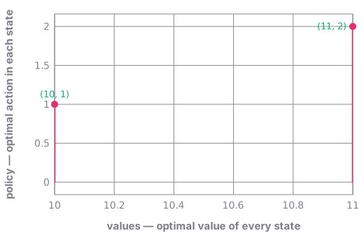
optimal action in each state, 1-based (the lowest-numbered one on a tie) (policy) at each optimal value of every state (values), both returned by optimization-ai999x for the worked example (R = [[1, 0], [0, 2]], T = [[1, 0], [0, 1], [0, 1], [1, 0]], gamma = 0.9): 10 → 1; 11 → 2.

The matrices of the worked example as heatmaps (rows and columns numbered; each cell shaded by its magnitude, negative values in the second colour; each panel shaded by its own largest magnitude): R (input); T (input); values (returned). Returned with them by optimization-ai999x: value_state_1 = 10. Other inputs: gamma = 0.9.

optimization_ai999x.solve('mdp_discounted', R=[[1, 0], [0, 2]], T=[[1, 0], [0, 1], [0, 1], [1, 0]], gamma=0.9)
# -> value_state_1 = 10, values = [10.0, 11.0], policy = [1.0, 2.0]   (SOLVED)

Questions in words (documented forms), as executed:

question	outcome	result
Solve the discounted Markov decision process with rewards [[1, 0], [0, 2]], transitions [[1, 0], [0, 1], [0, 1], [1, 0]] and discount factor 0.9.	SOLVED	value_state_1 = 10, values = [10.0, 11.0], policy = [1.0, 2.0]
Solve the discounted Markov decision process with rewards [[1, 0], [0, 2]], transitions [[1, 0], [0, 1], [0, 1], [1, 0]] and discount factor 1.	INVALID_INPUT	Discounted Markov decision process (optimal values and policy): the discount factor must be between 0 and 1 (exclusive).

Chromatic number (minimum graph colouring), graph_coloring

The fewest colours needed so that adjacent nodes get different colours (scheduling exams, assigning frequencies), and one such colouring.

$$\chi (G)=\min \{k:\mathrm{\exists }c:V\to \{\mathrm{1..}k\},c(u)\mathrm{\ne }c(v)\mathrm{\forall }uv\in E\}\backslash chi(G)\; =\; \backslash min\backslash \{k\; :\; \backslash exists\backslash ,\; c:\; V\; \backslash to\; \backslash \{1..k\backslash \},\backslash \; c(u)\; \backslash neq\; c(v)\backslash \; \backslash forall\; uv\; \backslash in\; E\backslash \}$$

input	meaning	condition
edges	edges 'A-B, B-C, ...' (undirected)

output	meaning
chromatic_number	minimum number of colours
coloring_example	one optimal colouring, in the order of 'nodes'
nodes	node order (first appearance)

• Method: exact backtracking for $k = 1$, 2, ... colours (largest degree first, symmetric colours skipped)
• Assumes: at most 14 nodes; no self-loops
• Evidence: certified procedure (gates: conditions, control, examples, fast_enough, questions, reference, sensitivity, templates)

one optimal colouring, in the order of 'nodes' (coloring_example) returned by optimization-ai999x for the worked example, one value for each position in the list (4 values, first 2, last 2, largest 3). Inputs: edges = A-B, B-C, C-A, C-D.

The network edges (edges 'A-B, B-C, ...' (undirected)) of the worked example (4 nodes, 4 edges, laid out on a circle); highlighted: the returned path A → B → C → D. Returned: chromatic_number = 3.

optimization_ai999x.solve('graph_coloring', edges='A-B, B-C, C-A, C-D')
# -> chromatic_number = 3, coloring_example = [2.0, 3.0, 1.0, 2.0], nodes = ['A', 'B', 'C', 'D']   (SOLVED)

optimization_ai999x.solve('graph_coloring', edges='A-B, B-C, C-D, D-A')
# -> chromatic_number = 2, coloring_example = [1.0, 2.0, 1.0, 2.0], nodes = ['A', 'B', 'C', 'D']   (SOLVED)

Questions in words (documented forms), as executed:

question	outcome	result
Find the chromatic number of the graph with edges A-B, B-C, C-A, C-D.	SOLVED	chromatic_number = 3, coloring_example = [2.0, 3.0, 1.0, 2.0], nodes = ['A', 'B', 'C', 'D']
Find the chromatic number of the graph with edges A-A, A-B.	INVALID_INPUT	Chromatic number (minimum graph colouring): a node cannot be joined to itself.

Minimum vertex cover (and maximum independent set), minimum_vertex_cover

The fewest nodes that touch every edge of a graph (placing guards or sensors), one such set, and the size of a largest set of pairwise non-adjacent nodes.

$$\tau (G)=\min \{\mathrm{\mid }C\mathrm{\mid }:C\cap \{u,v\}\mathrm{\ne }\mathrm{\varnothing }\mathrm{\forall }uv\in E\},\alpha (G)=\mathrm{\mid }V\mathrm{\mid }-\tau (G)\backslash tau(G)\; =\; \backslash min\backslash \{|C|\; :\; C\; \backslash cap\; \backslash \{u,\; v\backslash \}\; \backslash neq\; \backslash emptyset\backslash \; \backslash forall\; uv\; \backslash in\; E\backslash \},\backslash quad\; \backslash alpha(G)\; =\; |V|\; -\; \backslash tau(G)$$

input	meaning	condition
edges	edges 'A-B, B-C, ...' (undirected)

output	meaning
min_cover_size	size of a minimum vertex cover
cover_example	one minimum vertex cover
max_independent_set_size	size of a maximum independent set (nodes minus cover)

• Method: exact branch and bound (a node of largest degree in the cover, or all its neighbours)
• Assumes: at most 30 nodes; no self-loops; only nodes that appear in an edge count
• Evidence: certified procedure (gates: conditions, control, examples, fast_enough, questions, reference, sensitivity, templates)

The network edges (edges 'A-B, B-C, ...' (undirected)) of the worked example (5 nodes, 5 edges, laid out on a circle); highlighted: the returned path A → C → E. Returned: min_cover_size = 3, max_independent_set_size = 2.

optimization_ai999x.solve('minimum_vertex_cover', edges='A-B, A-C, A-D, B-C, D-E')
# -> min_cover_size = 3, cover_example = ['A', 'C', 'E'], max_independent_set_size = 2   (SOLVED)

optimization_ai999x.solve('minimum_vertex_cover', edges='A-B, A-C, A-D')
# -> min_cover_size = 1, cover_example = ['A'], max_independent_set_size = 3   (SOLVED)

Questions in words (documented forms), as executed:

question	outcome	result
Find the minimum vertex cover of the graph with edges A-B, A-C, A-D, B-C, D-E.	SOLVED	min_cover_size = 3, cover_example = ['A', 'C', 'E'], max_independent_set_size = 2
Find the minimum vertex cover of the graph with edges A-B, B-B.	INVALID_INPUT	Minimum vertex cover (and maximum independent set): a node cannot be joined to itself.